After going through this module, students will be familiar with the Euler and Runge-Kutta methods for numerical solution of systems of ordinary differential equations.  Examples are provided to show students how complementary R scripts can be written to help debug Runge-Kutta methods implemented in C++.

Contents

• Euler’s method (finite difference method)
• Using the Euler method to solve dN/dt = rho*N
• Implementing the Euler method in C++
• Comparison of the output of the C++ and R programs implementing the Euler method to solve dN/dt=rho*N
• Dynamic time step calculation in the Euler method
• Runge-Kutta method
• Example of implementation of Runge Kutta in C++: Lotka-Volterra predator prey model

Euler’s method (finite difference method)

From Wikipedia (because they say it well): “In mathematics and computational science, the Euler method is a first-order numerical procedure for solving ordinary differential equations (ODEs) with a given initial value. It is the most basic explicit method for numerical integration of ordinary differential equations and is the simplest Runge–Kutta method. The Euler method is named after Leonhard Euler, who treated it in his book Institutionum calculi integralis (published 1768–70).”

Say we would like to solve a system of one or more ordinary differential equations (here I give the example of two, but it could be just one, or more than two)

dx/dt = f(x,y)
dy/dt = g(x,y)

And assume the equations have initial conditions x(t_0)=x_0 and y(t_0)=y_0.

The first-order finite-time-step approximation to the differential equations is:

delta_x/delta_t = f(x,y)
delta_y/delta_t = g(x,y)

Moving the delta_t’s over to the other side yields:

delta_x = f(x,y)*delta_t
delta_y = g(x,y)*delta_t

And, assuming delta_x=x_(n+1)-x_n and delta_y=y_(n+1)-y_n:

x_(n+1) = x_n + f(x_n,y_n)*delta_t
y_(n+1) = y_n + g(x_n,y_n)*delta_t

To implement the Euler method, we employ an iterative process, where we start with the initial conditions x_0 and y_0, then calculate f and g at t_0, x_0, and y_0.  Then we would multiply f and g by delta_t, and add to the initial values of x and y to get the updated values.  Then the process is iterated for the desired length of time, or until some condition is met (for instance, until x or y is less than zero).

Using the Euler method to solve dN/dt = rho*N

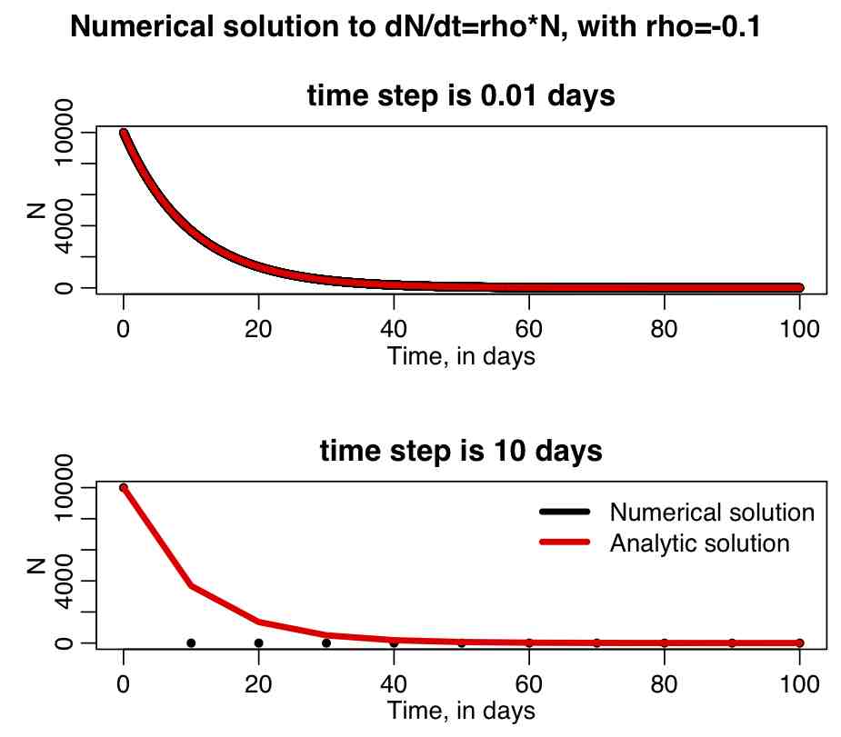
The R file euler_exp.R uses the Euler method to solve dN/dt=rho*N, with rho=-0.1, and the initial condition N_0=10,000.  If you run the script, it produces the following plot, which shows the numerical solution with a time step of 0.01 days (top), and the numerical solution with a time step of 10 days.  Overlaid in red is the analytic solution. Note that a large time step leads to a terrible approximation of the true solution!  How can you tell if your time step is too large?  Halve it, and rerun your simulation… if the numerical solution does not appreciably change, the time step is small enough.  If there is appreciable change, halve the time step again, and repeat the process over and over until the time step is small enough…

Implementing the Euler method in C++

The C++ program euler_exp.cpp does the same calculation, using the standard template libary.  Type g++ euler_exp.cpp -o euler and then type ./euler > euler.out

Comparison of the output of the C++ and R programs implementing the Euler method to solve dN/dt=rho*N

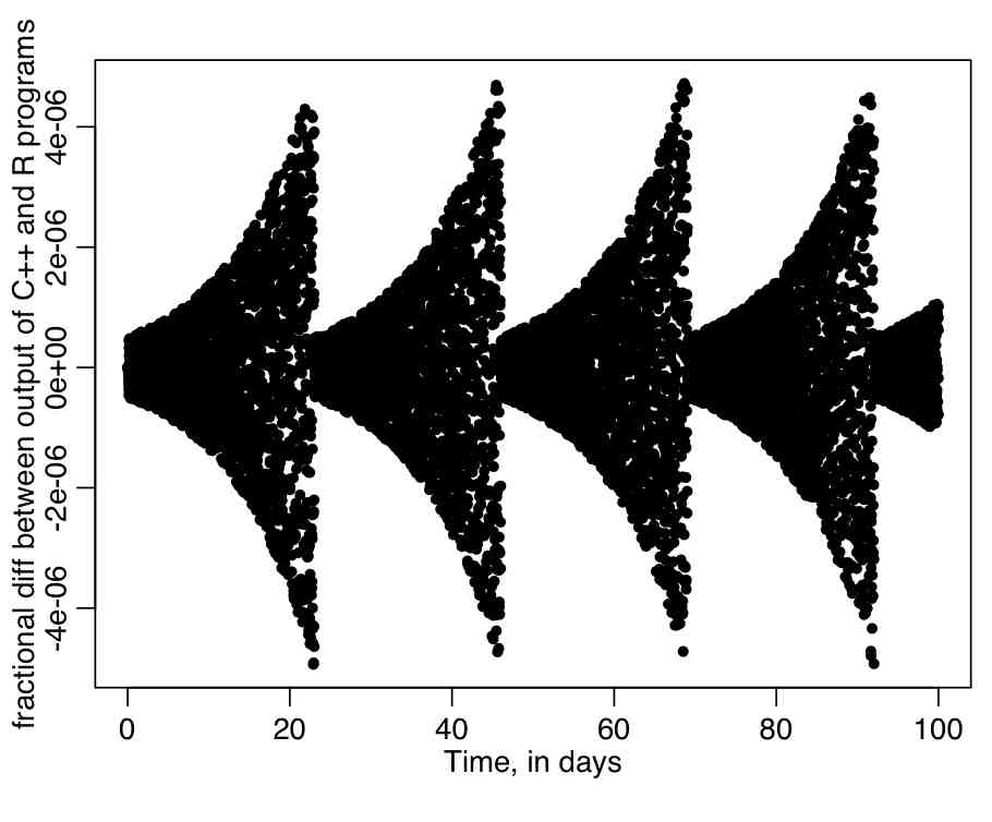
Then change the lread_cpp flag in euler_exp.R to be equal to 1, and rerun the euler_exp.R script.  It will calculate the fractional difference between the output of the calculations in the euler_exp.cpp program, and the output of the same calculation done in R. It will produce the following plot.  Do you think there is an appreciable difference between the results of the C++ and R programs?

Dynamic time steps in Euler method
There is no reason why the time step used in the Euler method needs to be constant.  In fact, more accurate solutions can be obtained if the time step is dynamically calculated to ensure that the overall change in the compartments is just one (or just a few).
To see how the dynamical time step would be calculated, consider the set of differential equations that describe births and deaths in two linked populations

x_(n+1) = x_n - alpha*x_n*delta_t + beta*y_n*x_n*delta_t
y_(n+1) = y_n - gamma*x_n*y_n*delta_t + delta*y_n*delta_t

We would like delta_t at time t_n to be small enough such that at most one individual is born or died. On average alpha*x_n individuals per unit time die in the x class, and beta*y_n*x_n are born. Similarly, in the y class on average gamma*x_n*y_n die and delta*y_n die per unit time. Thus the average number of births and deaths per unit time is A=(alpha*x_n+beta*y_n+gamma*x_n*y_n+delta*y_n). The time step needed to ensure that on average A is 1 is delta_t = 1/A.

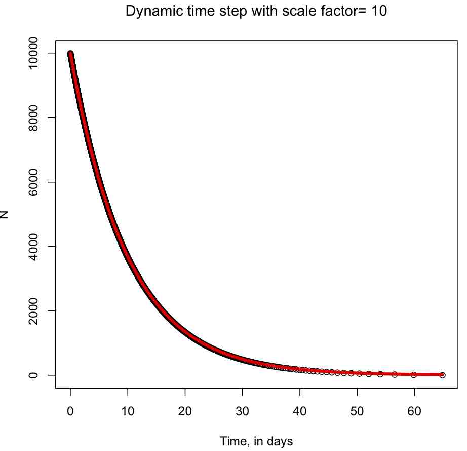
If A is large (as it would be for large populations, for instance), delta_t is tiny, and the calculations involved in the numerical solution could take a very long time. In reality, fairly good accuracy can usually be achieve by ensuring that the compartment changes at each step is less than some value, like 10 for instance.
The R script euler_exp_dynamic.R numerically solves dN/dt=rho*N with the Euler method using a dynamical time step calculation.  It produces the following plot (note that you can see the time step getting longer as N gets smaller):

Runge Kutta
The Runge Kutta method takes a sampling of four slopes through an interval and takes a weighted average to estimate the right end point.

 

Example of implementation of Runge Kutta in C++: Lotka-Volterra predator prey model

The Lotka-Volterra predator prey model has parameters

• a=birth rate of prey
• b=death rate of prey due to predation
• c=death rate of predators
• e=efficiency of turning prey into predators

(I don’t know what happened to d…)
If x is the prey, and y is the predators, the differential equations describing the time evolution of the populations is

dx/dt = a*x-b*x*y    and    dy/dt=e*b*x*y-c*y

The C++ header file PredatorPrey.h contains the class definitions of a class, PredatorPrey, that implements the Lotka-Volterra predator prey model.  The source code is contained in PredatorPrey.cpp.  An example of the use of this class is in example_predator_prey.cpp.  A makefile to compile the program is in makefile_lotka.  To compile the program, type

make -f makefile_lotka example_predator_prey

To run the program, and output the modelling results to a file lotka.out, type

./example_predator_prey > lotka.out

To determine if the output of the C++ program accurately models the predator prey system, we can compare the output in lotka.out to the output of the R dynamic time step Runge Kutta calculation using methods in the deSolve library.  This is done in example_predator_prey.R, which outputs the plot: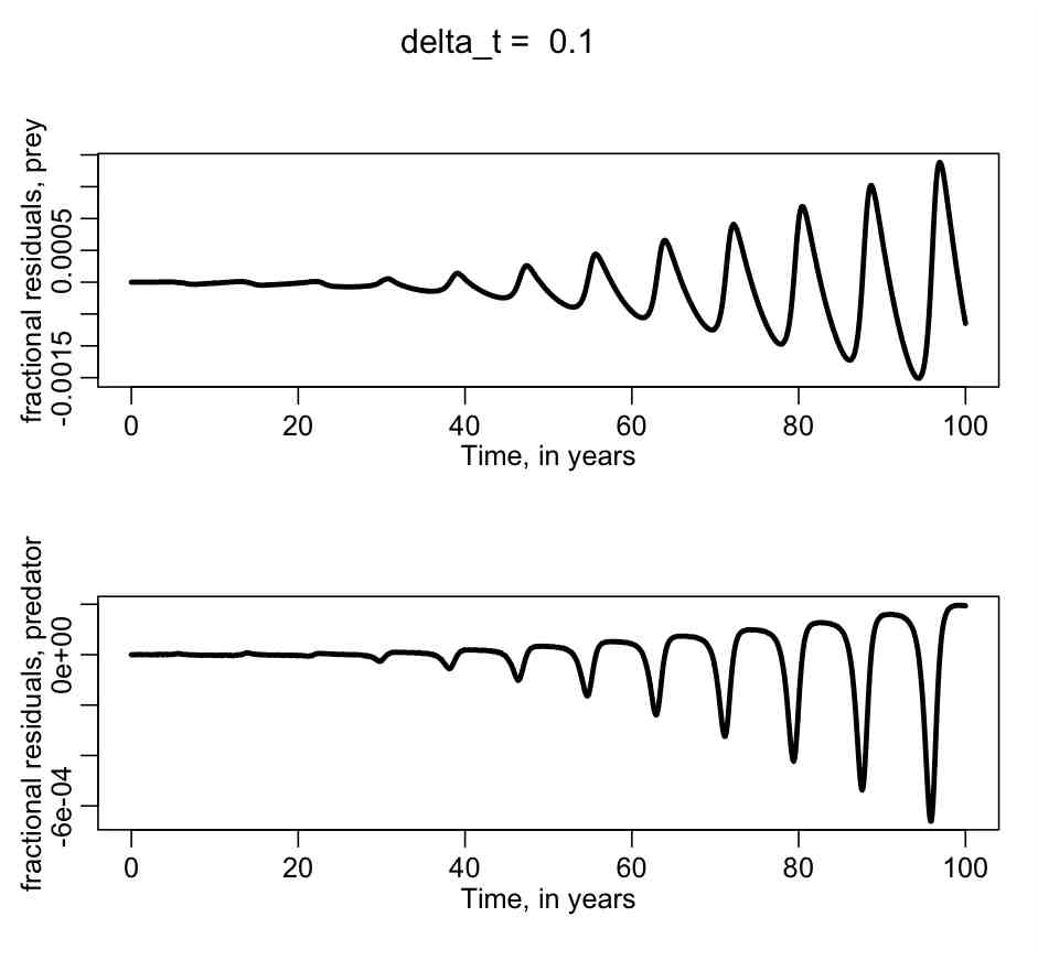
Do you think that the C++ program is doing a good job of accurately modelling the predator/prey system?