
Some (potentially) useful utilities for random number generation and manipulating vectors in C++
I’ve written some C++ code mainly related to vectors; calculating the weighted mean, running sum, extracting every nth element, etc). There are also utilities related to random number generation from various probability distributions, and methods to calculate the CDF of various probability distributions.
The file UsefulUtils.h and UsefulUtils.cpp contain source code of a class that contains these utilities that can be useful when performing compartmental modelling in C++. These utilities will be used extensively in the examples that will be presented in this, and later, modules. The file example_useful_utils.cpp gives examples of the use of the class. It can be compiled with the makefile makefile_use with the command
make -f makefile_use example_useful_utils
Homework #4, due April 3rd, 2013 at 6pm. The data for the homework can be found here.
The examples in the following discussion assume that the data are integer count data pertinent to some dynamical process like dynamics of interacting populations, disease spread, etc. If the data are not integer count data, but you have some idea of what the uncertainty, sigma_i, is on each observation, y^obs_i, you can calculate a Pearson chi-squared statistic as T = sum_i^N [(y^obs_i-y^pred_i)/sigma_i ]^2
If your data are not integer count data, and you have no idea what the sigma_i are, you are forced to assume that they are the same, and apply the Least Squares method for parameter estimation, using a random sampling procedure for the parameter hypotheses as described below. Estimation of the parameter uncertainties and their covariance matrix involves numerical estimation of the partial derivatives of the LS statistic wrt to the parameters near their best-fit values; this calculation is relatively straightforward.
The reason I do not present fitting methods involving gradient-descent algorithms here is because, in my experience, they don’t work well on real epidemic data because of multiple local minima in the figure-of-merit fitting statistic (in fact, in my experience, they’ve never worked with real data). There are non-linear optimization programs, such as Minuit, that employ a very sophisticated set of algorithms for minimization that will switch between methods as needed; while powerful, the disadvantage of using programs like Minuit for fitting the parameters of a non-linear dynamical model is that the model calculation for a particular set of parameter hypothesis takes up a great deal of computational overhead, over and above the large computational overhead involved in the Minuit fitting process. Combined with the fact that the optimization procedure cannot be done with parallel computing, this means that the optimization can take literally days to weeks of computing time, with no guarantee of having the parameters ultimately converge to a best-fit.
The methods I describe here involve a little bit of fiddling in the beginning to determine a good range of parameters for the random sweep, but the advantage of the initial steps is that you can visually compare the model to the data to ensure that it does indeed provide a reasonable description of the data. The next step involves coding up the algorithm in C++, checking that it is bug free, then submitting it in batch to a cloud computing system to perform the random sweeps in a massively parallel process that can yield fairly quick results. For simple models with only a few parameters that need to be determined, often cloud computing resources are not even needed; the fit can be done on a laptop overnight.
Fitting for the parameters of an SIR model: a fit to simulated data
When examining fitting to epidemic incidence data for an infectious disease whose spread can be described by an SIR model, the model parameters that are unknown are gamma (the recovery rate), the effective R0, the number of infected people in the population on day 0, I_0, and the fraction of the population that is immune to the disease on day 0, fimmune. Also unknown is the case detection rate, scale.
The R script SIR_generate.R generates the simulated over-dispersed incidence curve for a hypothetical disease spreading in a population of npop=250,000, with gamma=0.50, R0_eff=1.6, fimmune=0.20, I_0=250, and scale=0.05 (Note that initial conditions are also parameters of the model!!!). The simulated daily incidence over a 6 week period are output to a file SIR_simulated_epidemic_data.txt The file also makes the plot: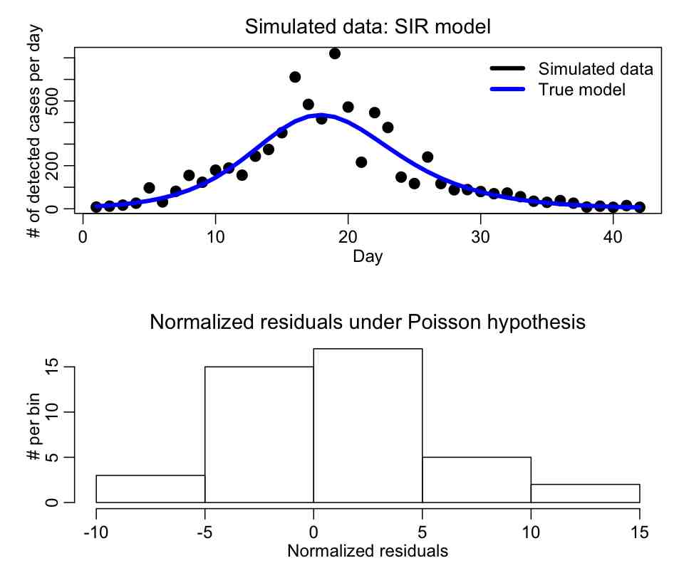
Do you think that the Pearson chi-squared method is applicable to fit to these data?
Begin the fitting process with initial exploratory studies in R:
The file SIR_initial_study.R reads in these data, and uniformly randomly samples parameter hypotheses for gamma, R0_eff, fimmune, and I_0 over a fairly wide range. For each set of parameter hypotheses, it calculates the Pearson chi-squared statistic, T. The random sampling procedure is repeated many times, and the resulting distributions of the Pearson chi-squared statistic (or negative log likelihood, if that is the kind of fit you are doing) vs the parameters are plotted (let’s refer to these as the figure-of-merit distributions). The best-fit solution is also overlaid on the data. The script, after running for a few hours, ultimately produces the following plot: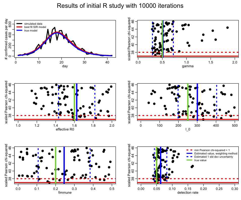
In an initial study like this, even though the figure-of-merit distributions will be somewhat sparsely populated, there are various criteria you are looking to fulfill:
- Do the data appear to be over-dispersed? If so correct the Pearson chi-squared for the over-dispersion (or switch to a Negative Binomial likelihood fit if you were using a Poisson likelihood fit). Once the figure-of-merit has been corrected, do you get a reasonable number of points lying in what you would expect to be the 95% CI of the parameter estimates (ie; between Tmin to Tmin+4)? If not, then you need to repeat the random parameter sweep process with more iterations. The problem may be that the range of the sweep for one or more parameters yields mostly poor fits to the data, in which case the ranges need to be adjusted.
- Does each parameter value corresponding minimum of the figure-of-merit statistic fall well within the range of the parameter sweep? If it is close to the edge (say, less than 3 std deviations away) then the range of the parameter sweep needs to be adjusted, and this initial step repeated.
- The range of the parameter sweeps also need to be adjusted if it is clear that a large portion of the range of a parameter does not yield a reasonable fit to the data.
- Does the best-fit solution appear to give a more or less reasonable description of the data? If not then you may have a bug in your code, or the model may simply be inappropriate for the data, in which case a different model should be employed.
- The one std deviation estimated CI on the parameters from the weighting method (blue dotted lines on the plot above) should more or less match up with the range of the points below min(T)+1. If they don’t, the parameter sweep ranges need to be made bigger and/or the number of iterations needs to be increased.
Given the plot above, what is your opinion of the range of the parameters used?
Next step: write C++ code to numerically solve the system of ODE’s for the SIR model, and test the code by comparing to the same calculation in R
The files SIR.h and SIR.cpp contain the source code to use the Runge Kutta method to solve the system of ODE’s for the SIR model. The file SIR_test.cpp is a test program that assumes some nominal parameter hypotheses, and outputs the resulting epidemic curve to a file. To compile this program, use the makefile makefile_sir and type
make -f makefile_sir SIR_test
To run the program, type
./SIR_test > SIR_test.out
The R script SIR_test.R reads in the output of the C++ program, and compares it to the same calculation in R using the methods in the deSolve library. The script produces the plot: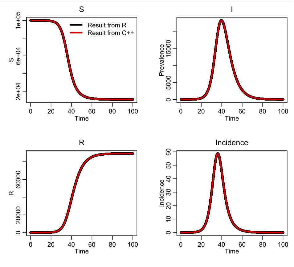
Next step: write a C++ program to read in the simulated data set, randomly sample parameter hypotheses, numerically calculate the predicted model, and calculate the Pearson chi-squared statistic comparing the model to the data.
The R script SIR_print_data_for_cpp.R prints out the simulated data in a format that is easy to copying and pasting into a C++ program.
The C++ files SimulatedDataSIR.h and SimulatedDataSIR.cpp implement a class that contains the simulated data. The program SIR_initial_fit.cpp implements this class, along with the UsefulUtils class, to fit an SIR model to the simulated data. The program SIR_initial_fit.cpp implements these methods. The makefile makefile_sir compiles the program, using the command
make -f makefile_sir SIR_initial_fit
To run the program, type
./SIR_initial_fit 0 > SIR_cpp_initial_fit.out
The R script SIR_step2.R reads in this file and plots the results: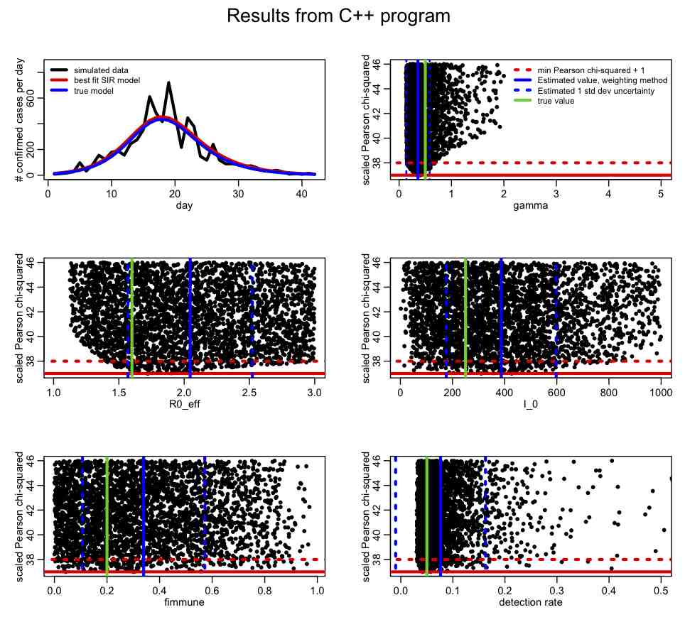
What is your opinion of the parameter ranges? How about the precision of the parameter estimates? In R, take a look at the correlation matrix, mycor. Which parameters appear to be the most correlated? Why do you think this is the case? Why do you think the estimates of the parameter one standard deviation uncertainties from the weighting method (blue dotted lines) don’t line up in some cases with the one-standard deviation estimates coming from the range of points under T<[min(T)+1]?
Incorporating parameter prior-information into the fit
For many models, information about the parameters and/or initial conditions can be obtained from other studies. For instance, for the SIR epidemic we’ve simulated, perhaps a serological study was done prior to the epidemic of some cross-section of the population, and the pre-immune fraction was estimated to be 0.22+/-0.05. Is this information independent from the epidemic data?
In order to incorporate this information into our fit, we assume that the pre-immune fraction is sampled from the Normal distribution, with mean 0.22 and standard deviation 0.05. This Normal distribution is the prior probability distribution for fimmune, and if we wish to incorporate this information as a constraint in our fit, we need to multiply our fit likelihood by this probability distribution.
Thus, to incorporate this prior information, we first correct (if necessary) the Pearson chi-squared statistic, T, for any over-dispersion. Then we add the term
[(fimmune-0.22)/0.05]^2
to the Pearson chi-squared statistic. This “prior-belief” correction is based upon the additive property of the chi-squared statistic. (side note: how many degrees of freedom does our resulting combined chi-squared statistic have? To calculate this, count the number of items of information going in to the fit, and subtract the number of parameters we are fitting for. Hint: the prior-information is one extra item of information going into the fit).
If you change the SIR_step2.R file to have lcorrect=1, it will apply this correction. This change produces the following plot: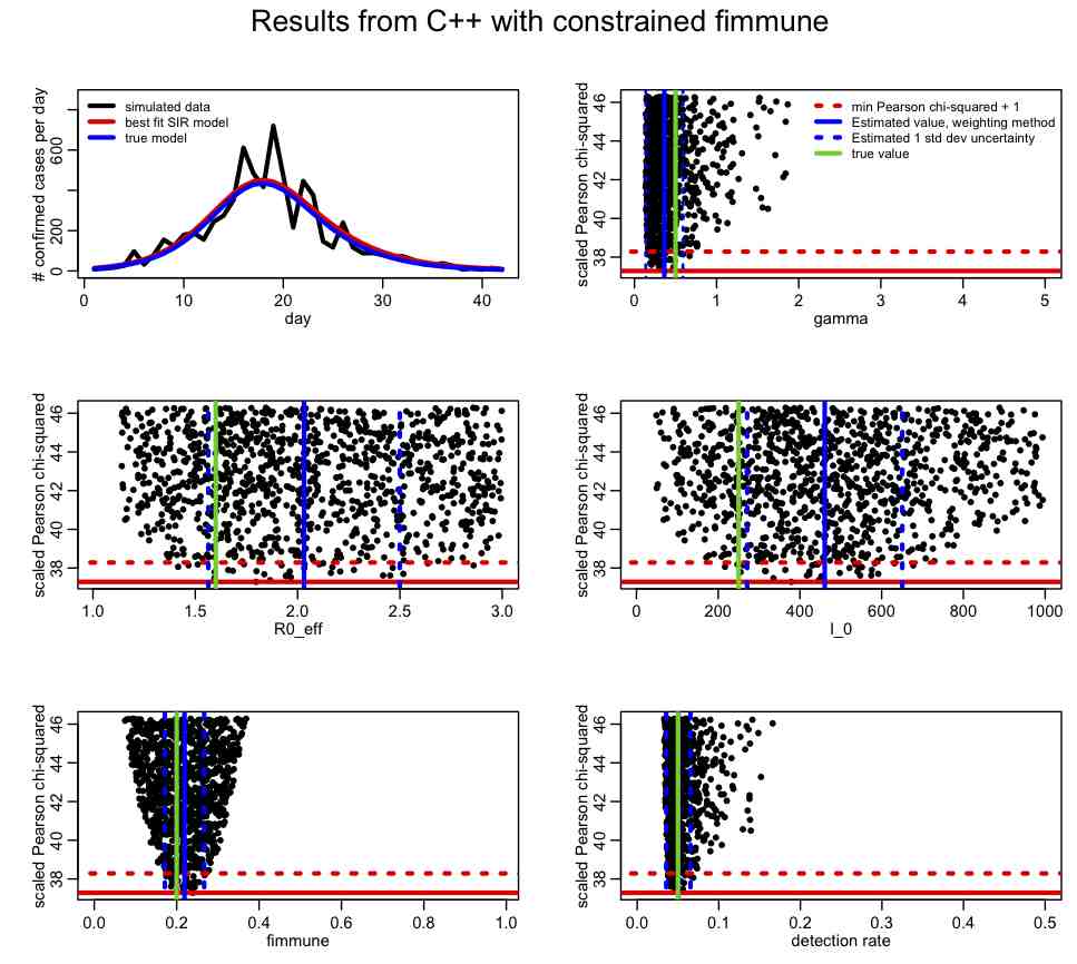
Compare this to the plot we produced above. How has the inclusion of the prior-information about fimmune help in our overall fit? Take a look at the correlation matrix, mycor. Which parameters are most correlated now?
For epidemic data, the recovery rate, gamma, is often know with some precision from observational studies of ill people. If you have an estimate of the recovery rate (with uncertainty) from such observational studies, you can incorporate that prior belief into the fit just as above. The following plot is made with SIR_step2.R with lconstrain=2, which incorporates prior-belief constrains on both fimmune and gamma: 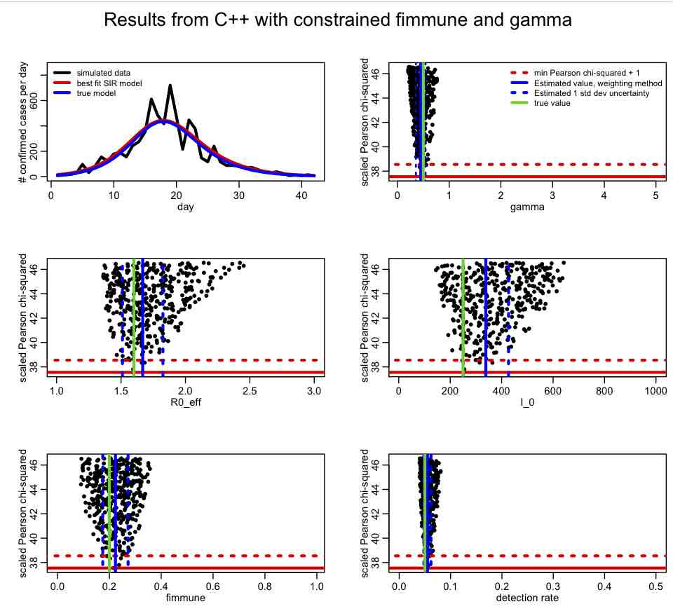
Has incorporating the prior-belief constraint on gamma helped to constrain the parameter estimates? Which ones?