Research in archaeoastronomy using computational, mathematical, and statistical methods, with free and open source software

[On this page I document and describe some of my work in archaeoastronomy, using mathematical, computational, and statistical methods to rigorously assess the probability that an archaeological site was used as an astronomical observatory.  I will give, as an example, all the programming code and other files I used to analyze a stone circle in the UK known as the “Merry Maidens”.]


Visits: 5440

AML 610 Module XIII: Canadian hare lynx data

Canadian Hare Lynx Data

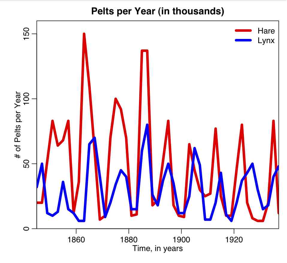
The file hare_lynx.txt contains data on the number of arctic hare and lynx pelts collected by the Hudson’s Bay company in Canada over the course of many years (data obtained from this website).  Do you think the Lotka-Volterra model is an appropriate model to fit to these data?

The R script hare_lynx_plot.R plots the Hare Lynx data:

hare_lynx

Continue reading

Visits: 2865

AML 610 Module XII: submitting jobs in batch to the ASU Saguaro distributed-computing system

The ASU Advanced Computing Center (A2C2) maintains the Saguaro distributed computing system, that currently has over 5,000 processor cores.

ASU students in the spring semester of AML610 should have already applied for and received an account on the Saguaro system (per the instructions of last month’s email describing how to apply for an account).

Saguaro allows you to simultaneously run multiple jobs in batch, directing standard output to a log file.  For this course, we will be using Saguaro to solve a system of ODE’s under a hypothesis for the parameters and initial conditions values (either chosen in a parameter sweep, or randomly chosen within some range); the output of the ODE’s will then be compared to a data set, and a best-fit statistic (like Least Squares, Pearson chi-squared, or Maximum likelihood) computed.  The parameter values and best-fit statistics are then printed to standard output.

Access to cloud computing resources, and knowledge of how to utilize those resources, has many different potential applications in modelling.  Learning how to use Saguaro as a tool in solving problems related to this course can thus potentially open up many further avenues of future research to you.

Homework #5, due Thus April 18th, 2013 at 6pm. Data for the homework can be found here.

Continue reading

Visits: 1304

AML610 module XI: practical problems when connecting deterministic models to data

Some (potentially) useful utilities for random number generation and manipulating vectors in C++

I’ve written some C++ code mainly related to vectors; calculating the weighted mean, running sum, extracting every nth element, etc).   There are also utilities related to random number generation from various probability distributions, and methods to calculate the CDF of various probability distributions.

The file UsefulUtils.h and UsefulUtils.cpp contain source code of a class that contains these utilities that can be useful when performing compartmental modelling in C++. These utilities will be used extensively in the examples that will be presented in this, and later, modules.  The file example_useful_utils.cpp gives examples of the use of the class.  It can be compiled with the makefile makefile_use with the command

make -f makefile_use example_useful_utils

Homework #4, due April 3rd, 2013 at 6pm. The data for the homework can be found here.

Continue reading

Visits: 4614

Numerical methods to solve ordinary differential equations

After going through this module, students will be familiar with the Euler and Runge-Kutta methods for numerical solution of systems of ordinary differential equations.  Examples are provided to show students how complementary R scripts can be written to help debug Runge-Kutta methods implemented in C++.

Contents

Continue reading

Visits: 7292

ASU AML 610 Module IX: Introduction to C++ for computational epidemiologists

After going through this module, students should be familiar with basic skills in C++ programming, including the structure of a basic program, variable types, scope, functions (and function overloading), control structures, and the standard template library.

So far in this course we have used R to explore methods related to fitting model parameters to data (in particular, we explored the Simplex method for parameter estimation).  As we’ve shown, parameter estimation can be a very computationally intensive process.

When you use R, it gives you a prompt, and waits for you to input commands, either directly through the command line, or through an R script that you source.  Because R is a non-compiled language, and instead interprets code step-by-step, it does not have the ability to optimize calculations by pre-processing the code.

In contrast, compiled programming languages like C, java, or C++ (to name just a few) use a compiler to process the code, and optimize the computational algorithms.  In fact, most compilers have optional arguments related to the level of optimization you desire (with the downside that the optimization process can be computationally intensive).  Optimized code runs faster than non-optimized code.

Continue reading

Visits: 1671

Fitting the parameters of an SIR model to influenza data using Least Squares and the graphical Monte Carlo method

[After reading this module, students should understand the Least Squares goodness-of-fit statistic.   Students will be able to read an influenza data set from a comma delimited file into R, and understand the basic steps involved in the graphical Monte Carlo method to fit an SIR model to the data to estimate the R0 of the influenza strain by minimizing the Least Squares statistic.  Students will be aware that parameter estimates have uncertainties associated with them due to stochasticity (randomness) in the data.]

A really good reference for statistical data analysis (including fitting) is Statistical Data Analysis, by G.Cowan.

Contents:

Introduction

When a new virus starts circulating in the population, one of the first questions that epidemiologists and public health officials want answered is the value of the reproduction number of the spread of the disease in the population (see, for instance, here and here).

The length of the infectious period can roughly be estimated from observational studies of infected people, but the reproduction number can only be estimated by examination of the spread of the disease in the population.  When early data in an epidemic is being used to estimate the reproduction number, I usually refer to this as “real-time” parameter estimation (ie; the epidemic is still ongoing at the time of estimation).

Continue reading

Visits: 25677

Basic Unix

In the Arizona State University AML610 course “Computational and Statistical Methods in Applied Mathematics”, we will be ultimately be using super computing resources at ASU and the NSF XSEDE initiative to fit the parameters of a biological model to data.  To do this, it is necessary to know basic Unix commands to copy, rename, and delete files and directories, and how to list directories and locate files.  We will also be compiling all our C++ programs from the Unix shell, and in the command line directing the output of our programs to files.
Continue reading

Visits: 1352

Good programming practices (in any language)

Easy readability, ease of editing, and ease of re-usability are things to strive for in code you write in any language. Achieving that comes with practice, and taking careful note of the hallmarks of tidy, readable, easily editable, and easily re-usable code written by other people.

While I’m certainly not perfect when it comes to utmost diligence in applying good programming practices, I do strive to make readable and re-useable code (if only because it makes my own life a lot easier when I return to code I wrote a year earlier, and I try to figure out what it was doing).

In the basics_programming.R script that I make use of some good programming practices that ensure easy readability. For instance, code blocks that get executed within an if/then statement, for loops, or while loops are indented by a few spaces (usually two or three… be consistent in the number of indent spaces you use).  This makes it clear when reading the code which nested block of code you are looking at.   I strongly advise you to not use tabs to indent code.  To begin with, every piece of code I’ve ever had to modify that had tabs for indent also used spaces here and there for indentation, and it makes it a nightmare to edit and have the code remain easily readable. Also, if you have more than one or two nested blocks of code, using tabs moves the inner blocks too far over to make the code easily readable.

In the R script sir_agent_func.R I define a function.  Notice in the script that instead of putting all the function arguments on one long line, I do it like this:

SIR_agent = function(N         # population size
                    ,I_0       # initial number infected
                    ,S_0       # initial number susceptible
                    ,gamma     # recovery rate in days^{-1}
                    ,R0        # reproduction number
                    ,tbeg      # begin time of simulation
                    ,tend      # end time of simulation
                    ,delta_t=0 # time step (if 0, then dynamic time step is  implemented)
                    ){

This line-by-line argument list makes it really easy to read the arguments (and allows inline descriptive comments).  It also makes it really easy to edit, because if you want to delete an argument, it is simple as deleting that line.  If you want to add an argument, add a line to the list.

Descriptive variable names are a good idea because they make it easier for someone else to follow your code, and/or make it easier to figure out what your own code did when you look at it 6 months after you wrote it.

Other good programming practices are to heavily comment code, with comment breaks that clearly delineate sections of code that do specific tasks (this makes code easy to read and follow).  I like to put such comments “in lights” (ie; I put a long line of comment characters both above and below the comment block, to make it stand out in the code).  If the comments are introducing a function, I will usually put two or three long lines of comment characters at the beginning of the comment block; it makes it clear and easy to see when paging through code where the functions are defined.

In-line comments are also very helpful to make it clear what particular lines of code are doing.

A good programming practice that makes code much easier to re-use is to never hard-code numbers in the program.  For instance, at the top of the basics_programming.R script I create a vector that is n=1000 elements long.  In the subsequent for loop, I don’t have

for (i in 1:1000){}

Instead I have

for (i in 1:n){}

This makes that code reusable as-is if I decide to use it to loop over the elements of a vector with a different length.  All I have to do is change n to the length of the new vector.  Another example of not hard-coding numbers is found in the code associated with the while loop example.

As an aside here, I should mention that in any programming language you should never hard-code the value of a constant like π (as was pointed out in basics.R, it is a built-in constant in R, so you don’t need to worry about this for R code).  In other languages, you should encode pi as pi=acos(-1.0), rather than something like pi=3.14159.  I once knew a physics research group that made the disastrous discovery that they had a typo in their hard-coded value of pi… they had to redo a whole bunch of work once the typo was discovered.

Notice in the script that I have a comment block at the top of basics_programming.R that explains what the script does, gives the date of creation and the name of the person who wrote the script (ie; me).  It also gives the contact info for the author of the script, and copyrights the script.  Every script or program you write should have that kind of boilerplate at the top (even if you think the program you are writing will only be used by you alone… you might unexpectedly end up sharing it with someone, and/or the boilerplate makes it clear that the program is *your* code, and that people just can’t pass it off as their own it if they come across it).   It also helps you keep track of when you wrote the program.


Visits: 6926

The basics of the R statistical progamming language

[After you have read through this module, and have downloaded and worked through the provided R examples, you should be proficient enough in R to be able to download and run other R scripts that will be provided in other posts on this site. You should understand the basics of good programming practices (in any language, not just R). You will also have learned how to read data in a file into a table in R, and produce a plot.]

Contents:

Why use R for modelling?

I have programmed in many different computing and scripting languages, but the ones I most commonly use on a day to day basis are C++, Fortran, Perl, and R (with some Python, Java, and Ruby on the side).  In particular, I use R every day because it is not only a programming language, but also has graphics and a very large suite of statistical tools. Connecting models to data is a process that requires statistical tools, and R provides those tools, plus a lot more.

Unlike SAS, Stata, SPSS, and Matlab, R is free and open source (it is hard to beat a package that is more comprehensive than pretty much any other product out there and is free!).

Continue reading

Visits: 3995