[In this module, students will learn the basics of modeling population dynamics (births/deaths, disease spread, wars, predator/prey, economics, etc) using compartmental models. Several simple examples will be discussed, and associated R scripts will be provided.]

A compartmental model is a type of mathematical model (that is to say, a model that can be described by a set of mathematical equations) that simulates how individuals in different “compartments” in a population interact.  The people (or animals) in each compartment are assumed to be the same as all the other people (or animals) in that compartment.   The compartments of the model can either flow between each other (for instance live individuals can flow to a “dead” compartment with a certain rate, which is 1/lifetime), or they can interact (for instance, predators eat prey… the prey doesn’t “flow” into the predator class, but obviously the number of predators that can survive is related to the number of prey available for them to eat… and the survival of prey is obviously related to the number of predators around to eat them).

These rates of flow between compartments, and interaction rates between compartments, are known as the “parameters” of the model.  Often, many parameters of models of population systems can be obtained from observational studies of the species… for instance, observational studies can reveal the average lifetime of the species. We’ll also discuss a model for the spread of a disease below; the rate of going from the “sick” compartment to the “recovered” compartment is something that can be determined simply by observing how long, on average, people are sick.

Why would we want to simulate things like the spread of disease within a population, or predator/prey systems, or wars, or economic systems? Well, if you can get a model that simulates what is happening in reality now, you can change the parameters of that model to examine ‘alternate realities’.  As we will see below, this can be used to devise improved disease intervention strategies, optimize pest control, optimize fisheries, etc, etc, etc.

An example of a compartmental model: fox/rabbit predator/prey system

For instance, a compartmental model could be used to simulate the number of animals over time in a predatory/prey system like foxes and rabbits.  One compartment would be the predators (the foxes), and they would be assumed to all be the same, with the same death rate, birth rate, ability to catch prey, etc.  The other compartment would be the rabbits, and they would also all be the same and have the same probability of being caught by a foxes.  Assuming that all individuals within a compartment is the same is obviously an approximation… in reality, some might be sick, some might have more babies than others, etc.  The interesting thing about compartmental models is that, even with these simplifying approximations, we’ll see below that they can do a remarkably good job of simulating reality.

How do we go about, in practice, simulating interacting populations like foxes and rabbits with a compartmental model? The usual first step is to draw what is known as a compartmental diagram, where you use boxes to represent the compartments of the model, and arrows to show the flow between boxes. Like so: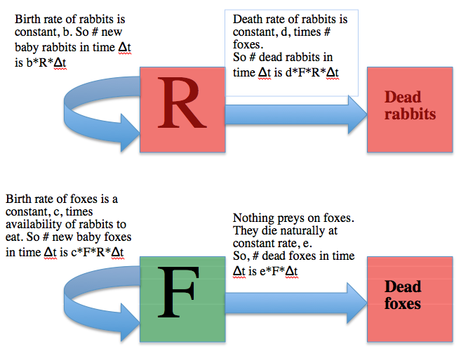 

Here’s the mathematical equations for the model: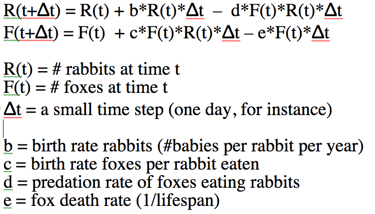

The two equations above are known as the Lotka-Volterra model, which was proposed in the early 1900’s as a way to simulate predator/prey interactions. The predators eating the prey, and the births and deaths in the model are known as the underlying model dynamics.  That is to say, the dynamics of the population that are captured by the mathematical equations of the model.

Note that the only way to estimate R(t) and F(t) at some time t with the above equations involves an iterative process that starts with some initial assumptions about the # of foxes and rabbits at time t=0, then at a small time step later uses those two equations to estimate R(t+delta_t) and F(t+delta_t).  Then, for the next time small step, set R(t) and F(t) to those values and calculate new estimates of R(t+delta_t) and F(t+delta_t).  You would continue iterating like that until you have estimates of R and F over the time span that you want to look at.

In the file fox_rabbit.R I have some simple code, written in the R programming language that implements the above iterative algorithm. R can be downloaded for free from their website. The R programming language can not only be used for computing algorithms like the one above, it also has nice plotting methods. I have written an online module on the basics of programming in R.  Note that I use R here to do these calculations, but you can just as easily code this algorithm up in Excel, or Matlab, or Maple, or Mathematica, or Java, C or C++.

In order to run the code in fox_rabbit.R, simply start up R and copy and paste the code into the command line.  It will produce the following plot:

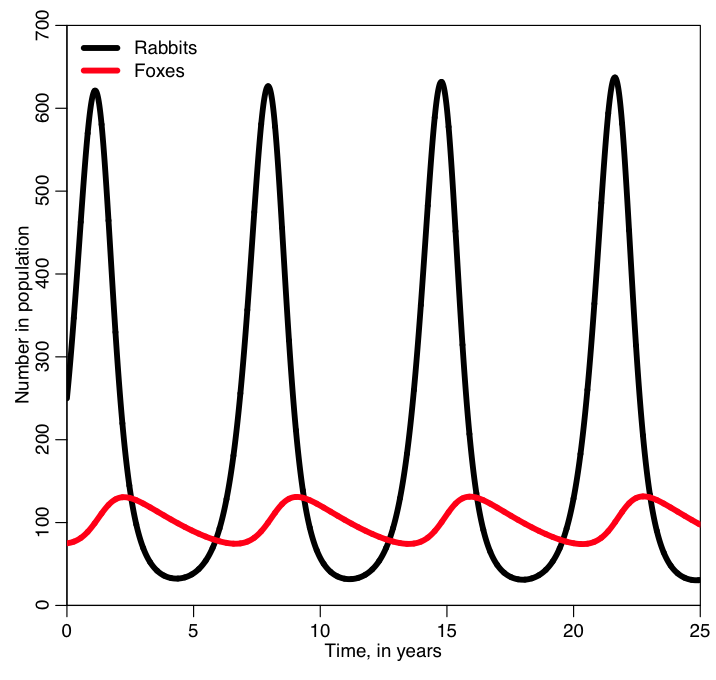
I bet you weren’t expecting the oscillations that we see in the two populations!  Why do you think the populations oscillate? And why do you think the peaks in the fox population are slightly out of phase with the peaks in the rabbit population?  What happens if you change the initial number of foxes and rabbits in the population and rerun the code?

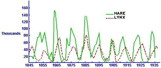
It turns out that oscillatory population sizes are seen in predator prey systems all the time.  For instance, here is a plot of data on the number of pelts of snowshoe hares and lynx collected by the Hudson’s Bay Company in Canada over several decades:

(figure from math.duke.edu)

I think it is very interesting how such a simple model can so accurately predict very complex dynamics.  I also think it is interesting that models like the Lotka-Volterra model, that we can only solve numerically, were developed long before computers were available to do the numeric simulations (!).

Explaining the oscillating behaviors that can be found in predator/prey systems is an example of the advantages of mathematical models over statistical models.  With a statistical model, we could regress the number of prey on the number of predators and you would likely find that they are uncorrelated… but there are obvious strong cyclical patterns in the system! The statistical model gives us no information as to why that is the case. The mathematical model includes the dynamics of the interplay between the two populations, and easily explains the patterns.

The advantages of using calculus and differential equations to describe a compartmental model

The Lotka-Volterra model, as I’ve described it above, doesn’t require any knowledge of calculus to solve, if you use the iterative method with a small time step (quick aside, what happens if you don’t make the time step small enough? And, how would you know if the time step you are using is small enough?).  I’ve written a past module on compartmental modeling without calculus.

With calculus, however, there are many different things that can be analyzed with the model like equilibrium points of population sizes and their stability, exponential rise in disease cases at the beginning of an epidemic (more on that below), phenomena like bifurcations and chaos, etc.  Much more common than the iterative algorithm I describe above is to express the model equations as a set of differential equations.  Compare this

to this

The system of differential equations can be solved with numerical methods, like the Runge Kutta method.  The R programming language has built-in functions that do that for you.

What does dR/dt=0 and dF/dt=0 imply?  For which values of F and R does that happen?

So, what do mathematical modellers do all day, anyway?

People in the field of mathematical modelling keep busy with a variety of things; if their research interest is compartmental modelling, primarily they come up with new compartmental models that try to optimally describe the underlying dynamics of a population or system, with the aim of getting an accurate description of what is observed in reality.

They do this sometimes by adding new compartments onto an already existing model (for instance, maybe they would add a second predator compartment onto the above model to take into account the fact that it isn’t just foxes that eat rabbits… or maybe there is a second prey compartment to take into account that foxes eat more than just rabbits).  By the way, in a model for the Canadian hare/lynx above, what extra effect would we probably need to take into account?

Or sometimes mathematical modellers might extend a standardly used model by making one or more of the model parameters vary in time. For instance, rabbits might only have their babies in the spring and summer, when there are lots of green things to eat.  Thus the birth rate for rabbits wouldn’t be a constant, it would be some kind of time-varying function that was low in winter and high in summer.

Mathematical modellers can also do things like change their model to reflect some kind of complexity they would like to add to the underlying system dynamics. For instance, maybe they would like to take into account in a disease model the vaccination of individuals (so they would add a “vaccinated” compartment of individuals to their model, and those individuals would be immune to the disease).  Often, with disease models, the idea is to get a model that simulates reality as we see it now, then design an optimal disease intervention method by making some changes to that model.

Sometimes mathematical modellers will think of an entirely new model to simulate something that no one has ever thought of modelling before.

Mathematical modellers will also do mathematical analysis of the system of equations of their model.  These kind of analyses can reveal a lot of interesting information about the system.  There is a summer undergraduate research program at Arizona State University called the Mathematical Theoretical Biology Institute (MTBI) where undergraduates who have two years of undergraduate math courses spend 8 intensive weeks listening to lectures and working on mathematical modelling research projects. The students at MTBI are no different than NEIU students (in fact, some have been NEIU students) in that they have a very diverse array of backgrounds and are of varying ages (it is not uncommon for mature students to take part in the programme). Many of the MTBI project papers have been published, and many of the students have won poster competitions and gone on to graduate school. I mentored a student group this past summer that used a compartmental model to simulate cyber-bullying on Twitter.  They used their model to figure out how ways to suppress cyber-bullying.

People who work in the modelling field will also often employ computational models in addition to mathematical models, like agent-based models or other stochastic models, to simulate dynamic systems.  Often these models don’t have a mathematical equation for the dynamics that you can write down, but do have an algorithm for simulating the dynamics that you can describe and implement in computer code. I’ve written a past module about stochastic simulation methods (like agent based models).

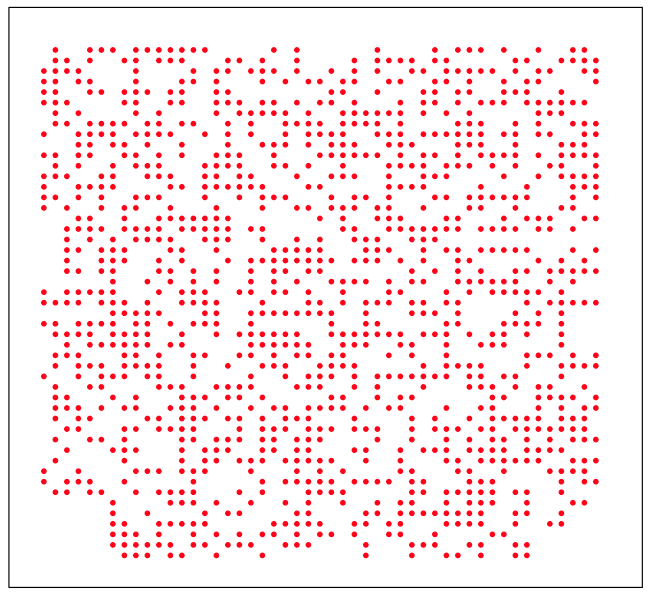
For instance, we could use an agent based model to simulate a population that competes for resources with its neighbors on a grid (an example of this would be trees in a forest, or saguaro cactuses in the desert).  We start the simulation with individuals evenly spaced on a square grid, and at each time step an individual is randomly chosen on the grid.  That individual randomly choses one of its neighbors (if it has any left) and then eats that neighbor. I’ve implemented this algorithm in the file agent_grid_eat.R.  An example of the final plot produced by this script is: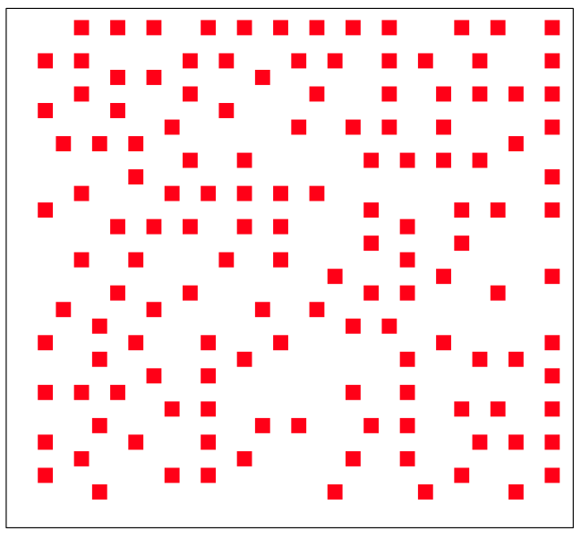

The resulting spacing of the individuals on the grid might look pretty random, but in reality it isn’t very random (it is actually remarkably even).  A true randomly spaced grid is implemented in grid_random.R, and looks (for instance) like this: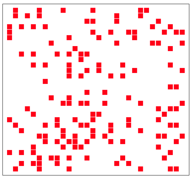

Can you see the qualitative difference?

Another example of the use of an agent based model is the simulation of development of hair follicle cells during fetal development.  The hair on our bodies is not randomly distributed (otherwise, just like in the plot above we would have scattered bald patches on our head).  Roughly summarized, current prevailing theory has it that during fetal development cells on the skin turn into hair follicle cells, then send chemical signals to try to convince their neighbouring cells to do the same.  The neighbouring cells (essentially) have some probability of saying no.  So, the hair follicles spread kind of like a rash over the head, but not all cells on the head end up being hair follicles.  I’ve written an R script called agent_grid_hair.R that simulates this process.  It produces the plot:

Other examples of computational models are finite element analysis models in engineering and biomedical engineering where they break up an object into small representative bits, and then analyze the changing forces on each element as the object moves or has forces applied to it.

 

Physicists and engineers also use computational models to examine fluid and gas flows, for example, when trying to design an optimal rocket shape.  They also use computational models for modelling forest fires

I am not only a mathematical and computational modeller but also a statistician; my primary research interest in the field of mathematical modelling is fitting the parameters of compartmental models to data, because not all the parameters of the model can be obtained by observing the population… some parameters have to be estimated.  The way I do this is I try many different parameter values, and look for the set of parameter values that gives a model prediction that best matches some data I have.  The idea is simple, but it carrying out the necessary calculations is computationally intensive.  I typically use super-computers to do these calculations.  Doing what I do isn’t hard.  It just takes some computing background and a basic (although somewhat specialized) knowledge of statistics.  I teach a one semester online course in the methods that I use.

Mathematical modellers not only work in academia, but also in industry and for the government.

On to another compartmental model example: modelling warfare

Another simple example of the use of compartmental models is modelling warfare between two sides (the A=”Reds” and the B=”Blues”) using what is known as a Lanchester model (again, this model was developed in the early 1900’s).  The model differential equations look like this:

dA/dt = -βB

dB/dt = -αA 

where alpha is the rate at which the A’s can shoot at (and kill) the B’s, and beta is the rate at which the B’s can shoot at (and kill) the A’s. Do the number of people in the armies ever go up?

There is an exact solution to the above equations (ie; you don’t have to solve them numerically), but it is pretty nasty looking.  In the R script lanchester.R I simulate a war between two small armies using the same simple iterative approach to solve the equations that we used for our fox/rabbit example.  You can copy and paste the contents of the script into the command line in R to run it.

In the program, army A starts off with 40 people, and each person in that army can kill twice as many people per day as someone in army B.  But army B starts off with 50% more people (they start off with 60).  Which army do you think will win?

The script produces the following plot:

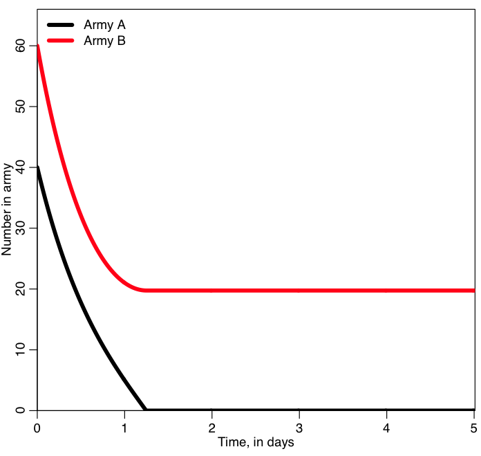
Who won?  was it who you expected to win?  What do you think will happen if you start with A=400 and B=600?

An extension of the Lanchester model is known as the Salvo model, and takes into account that not only the shooting rates of the armies, but also how many “hits” a member of an army would have to take to be out of commission (“killed”).  A member of the army in this case might be a warship.  With this kind of model, an army can do various cost/benefit studies;  do they want to invest in being able to shoot faster (and/or with greater deadliness), or do they want to invest in better armor for themselves?

Modelling of diseases

Compartmental models lend themselves really well to simulating the spread of disease in a population.  Models of disease spread can yield insights into the mechanisms and dynamics most important to the spread of disease (especially when the models are compared to epidemic data).  With this improved understanding, more effective disease intervention strategies can potentially be developed. Sometimes disease models are also used to forecast the course of an epidemic or pandemic.

The bread-and-butter of compartmental disease models is the Susceptible, Infected, Recovered model developed by Kermack and McKendrick (again, in the early 1900’s).  This remarkably simple model works very well for many diseases like mumps, measles, rubella and influenza (for instance).

With the SIR model, you start with a population of N people.  Most of the people are in the “susceptible” compartment and are susceptible to some disease (say, influenza) because they have no immunity to it.  Initially a few infected people are infected with the disease an are put into an “infected” compartment.  The entire population mixes homogeneously (meaning that the people an individual contacts each day are completely random).  During the duration of their illness the infectious people each infect on average X susceptible people, who then flow into the infected compartment (thus, the susceptible compartment flows into the infected compartment).  These newly infected people each then go on to and infect X other people, and so on, and so on, and so on (for a disease like influenza, X is around 1.5… for a disease like measles, X is around 10).

Can you see that the number of infected people in the population will initially grow exponentially?  In fact, it can be shown that the exponential growth rate is equal to (X-1) divided by the length of the infectious period. In a moment, we will show this property of initial exponential rise using the model equations.

Eventually, after some period of time known as the “infectious period” or “recovery period”, the people recover and for many diseases (but not all!) they are immune to the disease.  The infectious compartment thus flows into a “recovered” compartment.  Individuals in the recovered compartment don’t flow out of it (if the immunity upon recovery is permanent).

Here is what the compartmental diagram looks like:

Notice that nothing flows into the S compartment (because we don’t have births in the model). The model equations are:

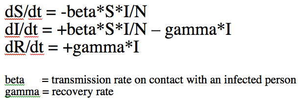
These equations can only be solved numerically (for instance, by using the iterative time step method we’ve talked about).

When an epidemic begins in an almost completely susceptible population, S is approximately equal to N.  Thus the equation for dI/dt is approximately

The solution to this equation is

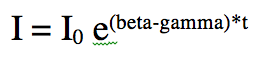
Thus, we see that indeed, the rate of rise at the beginning of the epidemic is exponential.  We will be returning to the topic of initial exponential rises of epidemics in the next module.

Even though the initial rise in infected cases is exponential, it doesn’t continue that way… after a while, a significant fraction of the population becomes recovered and more and more people that an infected person contacts during their infection is recovered and immune.  Recall from your Calculus I course that when a function is at its maximum or minimum, the first order derivative of the function is zero.  Thus, to find the point when I is maximal, we can set dI/dt=0 in the equations above, and solve for S.  This yields that I is maximal when S/N=gamma/beta.  It turns out that beta/gamma is a very special quantity known as the “Reproduction Number” of the disease, R0 (aka: “R naught”).  It is the average number of people that an infectious person infects during the course of their illness if they are in a completely susceptible population.

As an aside, for what other value of I is dI/dt=0?

In the file sir_simple.R, I use the iterative method I described above to solve the SIR system of equations for a hypothetical epidemic where the recovery period is 1/gamma=7 days, and R0=7 (so beta = R0*gamma = 1). The population size is 1000.  It produces the following plot: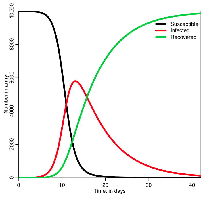

Was the behavior of the three lines what you expected?

 

There are lots of ways you can extend the simple SIR model.  For instance, here is an example of a compartmental diagram for a bit more complicated model that includes births and deaths:(From CU Boulder Applied Math Biology Group)

How would you modify the SIR model equations to include births and deaths as indicated in the above diagram?

If you want more information about compartmental modelling of epidemics, I’ve written several past modules on epidemic modelling using the SIR model and various extensions.  See here, here, and here.