In this talk, I’ll discuss several past analyses I’ve done with collaborators where we have combined statistical and mathematical modelling methods to explore some interesting research questions.

I’m a statistician, and I also have a PhD in experimental particle physics.  Research in experimental particle physics can involve complex models of observable physical processes, and fitting of those models to experimental data is a not uncommon task in that field.  Like the field of applied mathematics in the life and social sciences (AMLSS), the models being fit at times have no analytic solution, and must be solved numerically using specialized methods.  When I entered the field of AMLSS back in 2009, I had a lot to learn about the various models used in this field and the common methodologies, but I already had a solid tool box of specialized skills that allowed me to connect mathematical models to data, and it has turned out that those skills have been remarkably useful in exploring a wide range of research questions in the life and social sciences that I find interesting.  I also apply these skills in consulting projects I do.

First off: what is the difference between statistical and mathematical modelling, anyway?

The difference between statistical and mathematical models is often times confusing to people.  In this past module on this site, I discuss an example of the differences, with an analysis of seasonal and pandemic influenza used as an example.

Example of an analysis combining statistical and mathematical modelling: Mathematical and statistical modelling of the contagious spread of panic in a population

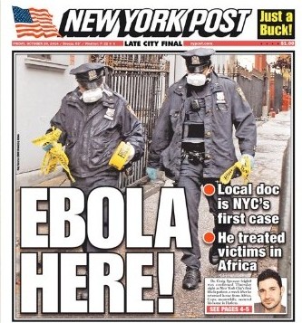
During the 2014 Ebola outbreak, there were a total of five cases that were ultimately identified in America, compared to tens of thousands of cases in West Africa.  Even though the “outbreak” in America was essentially non-existent, once the first case was identified in the US in autumn 2014, the media shifted into 24/7 coverage of the supposed dire threat Ebola presented to Americans, complete with scary imagery.

Autumn 2014 I was teaching a course in the ASU AMLSS graduate program on statistical methods for fitting the parameters of mathematical models to data.  Each year, when I teach AML classes, I usually try to have a “class publication project” that encompasses the methodology I teach in the class.  In this case, I thought it might be interesting to try to model the spread of Ebola-related panic in the US population, as expressed on social media, and explore how news media might play a role in that.

The class did the analysis as a homework assignment, and we wrote the paper together, which was published in 2015.  The paper received national media attention when it came out.

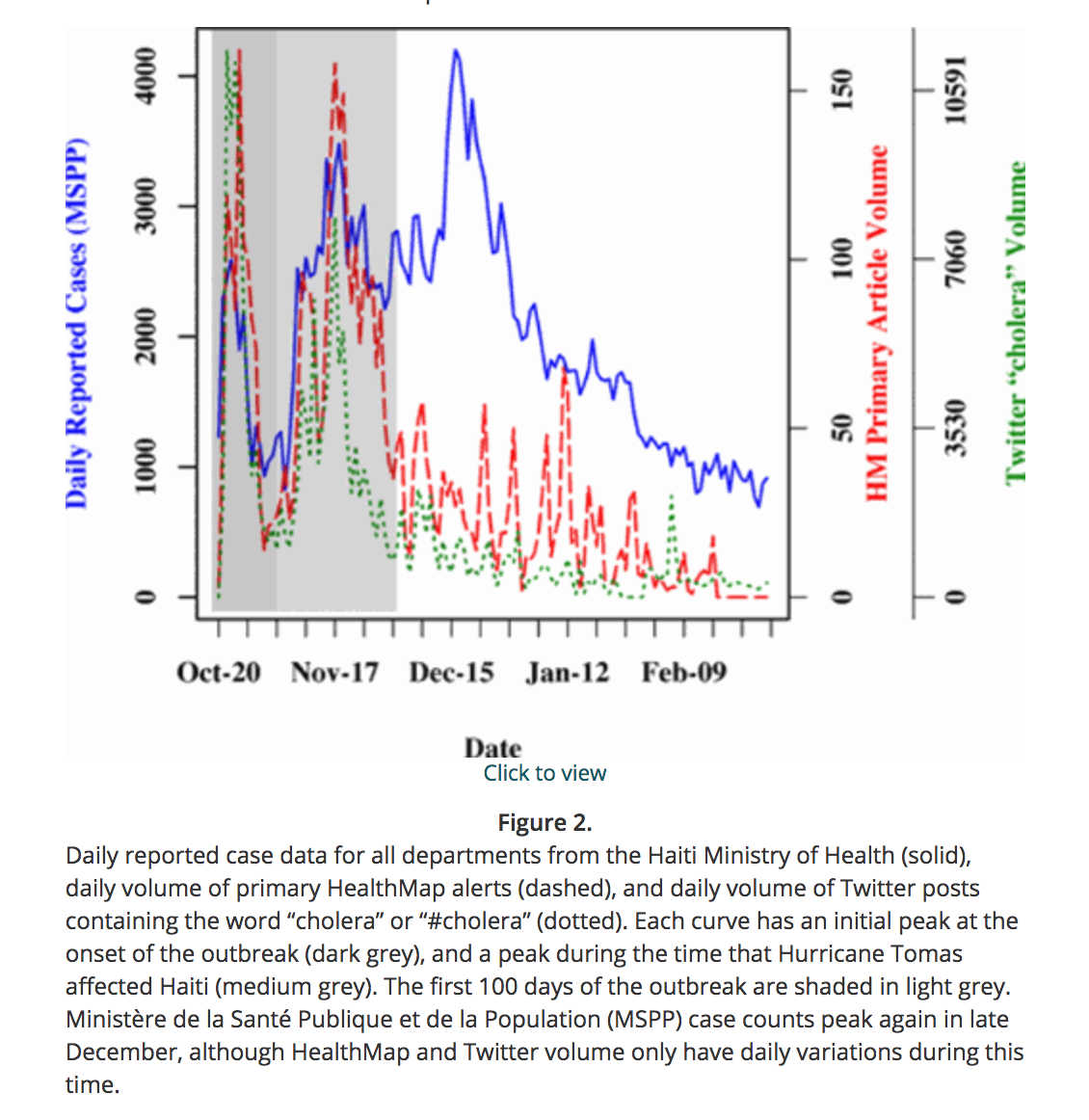
First; why was this analysis important?  Well, it has been suggested in the past that people talking about a particular disease on social media might perhaps be used as a real-time means to assess the temporal and geospatial spread of the disease in the population, rather than relying on slower traditional surveillance methods, which can suffer from backlogs in laboratory testing.  For instance, tracking influenza, or cholera:

However, up until the US Ebola “outbreak” the problem was that it was impossible to say whether people were just discussing a disease on social media because they were worried about it, rather than because they actually had it.  During the Ebola outbreak, pretty much no one actually had it in the US, so everyone who was talking about it was doing so because they were concerned about it.  This gave us the perfect instance to gauge what kind of temporal patterns we might see in social media chatter due simply to panic or concern about a disease!

The data we used in the study were the daily number of news stories about Ebola from large national news outlets.  We also obtained Twitter data related to Ebola, and Google search data in the US with search terms related to Ebola, including “do I have Ebola?” from Google Trends. Here is what the data looked like:

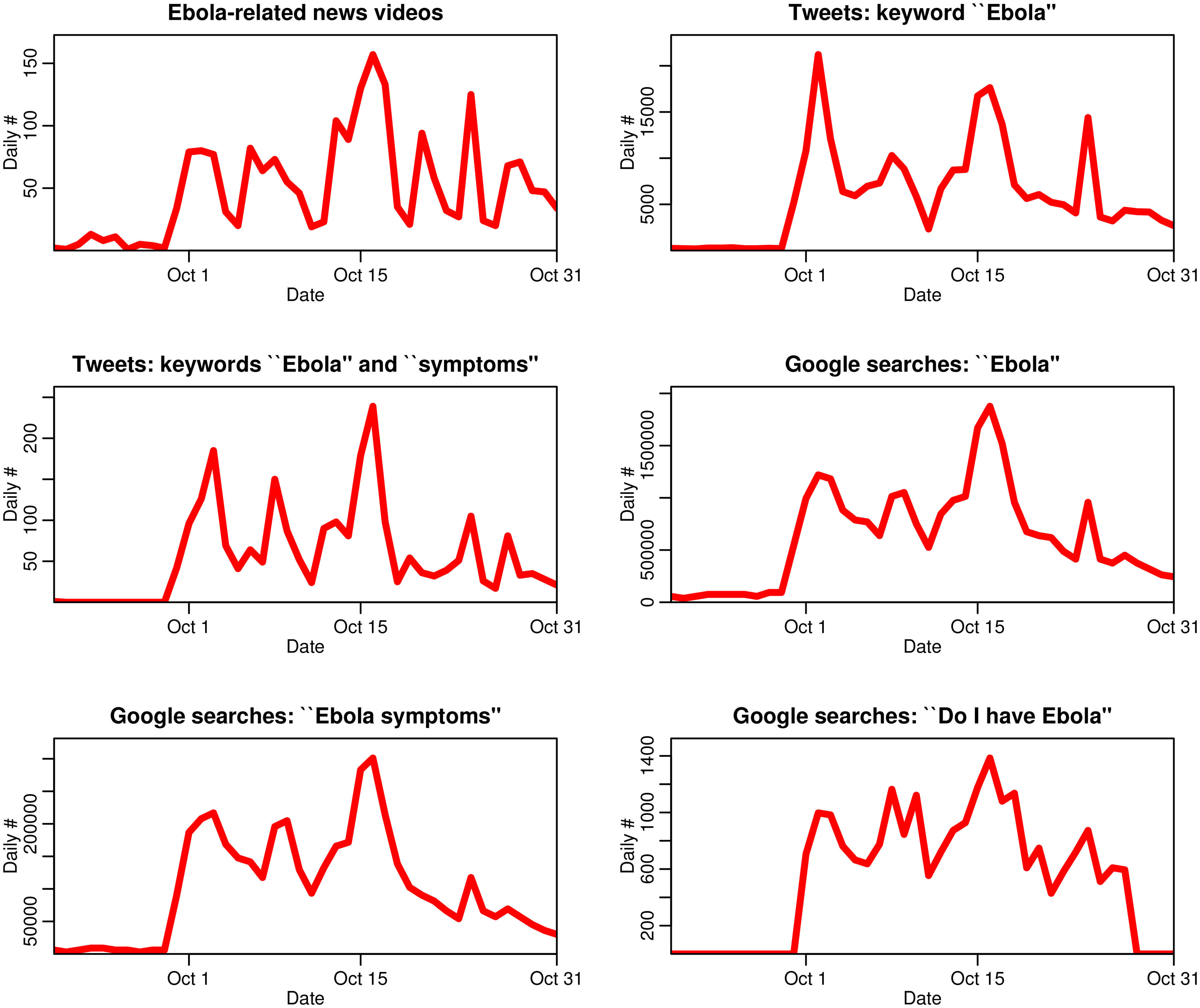
We came up with a model that related the number of news videos, V, and people who were infected, I, with the idea to tweet about Ebola, or do a Google search related to Ebola:

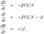
The parameter beta is a measure of how many tweets (or Google searches) per person per unit time one news story would inspire, and gamma parameterizes the “boredom” effect, through which people eventually move to a “recovered and immune” class, upon which they never tweet again about Ebola no matter how many Ebola-related news stories they are exposed to.  Using the statistical methodology taught in the AML course, the students fit the parameters of that model to data, and obtained the following model predictions, shown in red:

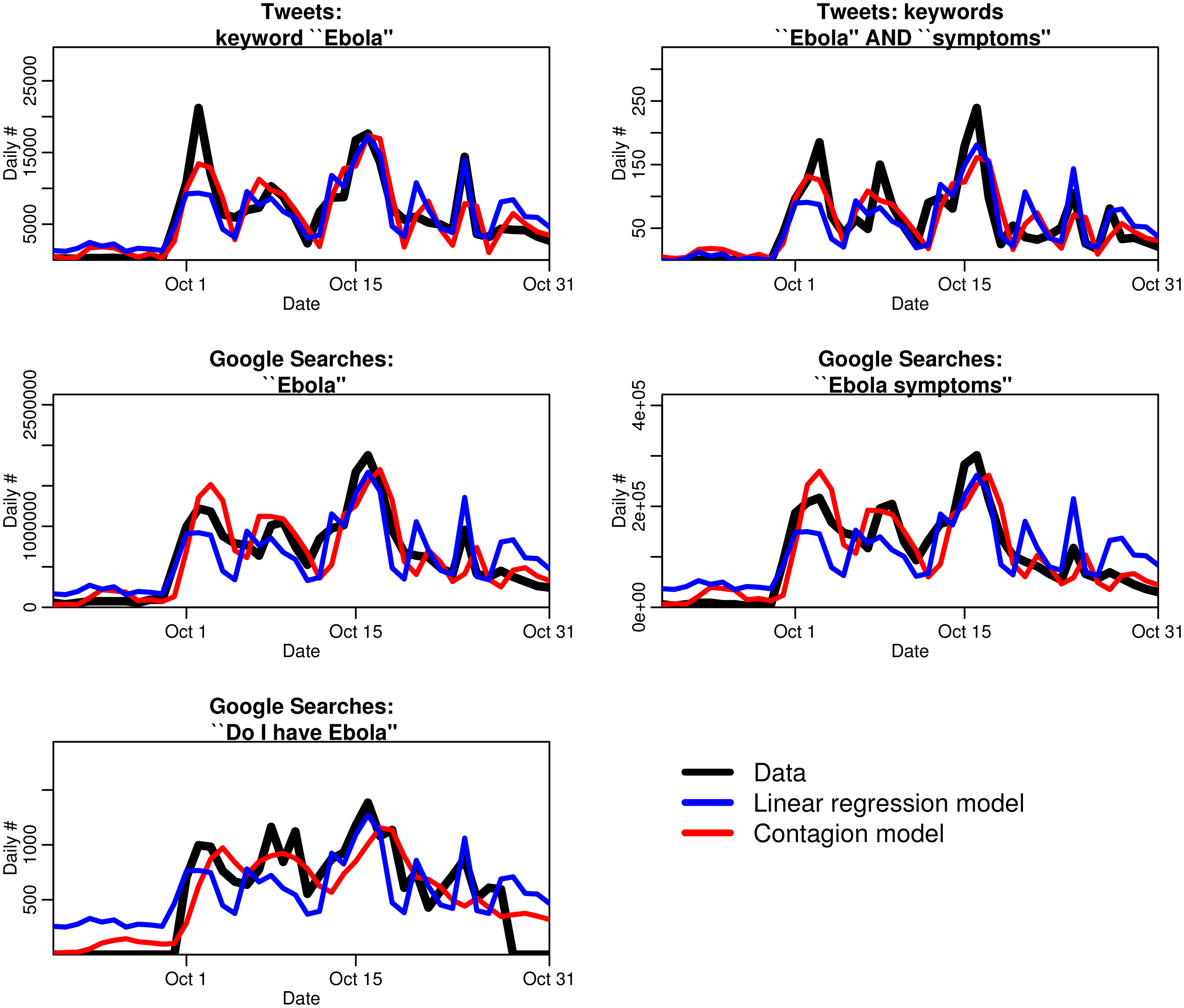
The blue lines on the plot represent a plain statistical model that simply regresses the Twitter and Google search data on the news media data, without taking into account the “boredom” effect.  Can you see that the regression fits are systematically too high early on, and systematically too low later for all the plots, but the same is not true of our mathematical model?  That tells us that our mathematical model that includes boredom really does do a better job of describing the dynamics of peoples’ Ebola-related social media behaviours!

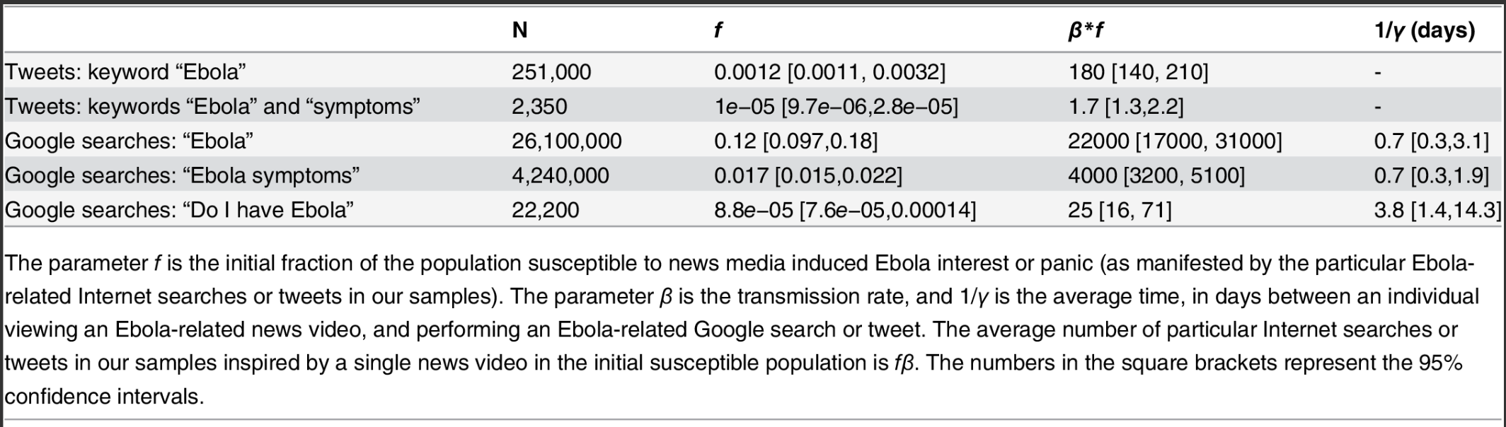
We found that each Ebola-related new story inspired on average thousands of tweets and Google searches. Also, on average, we found people were only interested enough for a few days to tweet or do Google search after seeing a news story about Ebola before they became bored with the topic:

We couldn’t have done this analysis without both mathematical modelling and statistical methods; it was a nice “bringing together” of the methodologies to explore an interesting research question.

Another example of an analysis that involved mathematical and statistical modelling methods: contagion in mass killings and school shootings

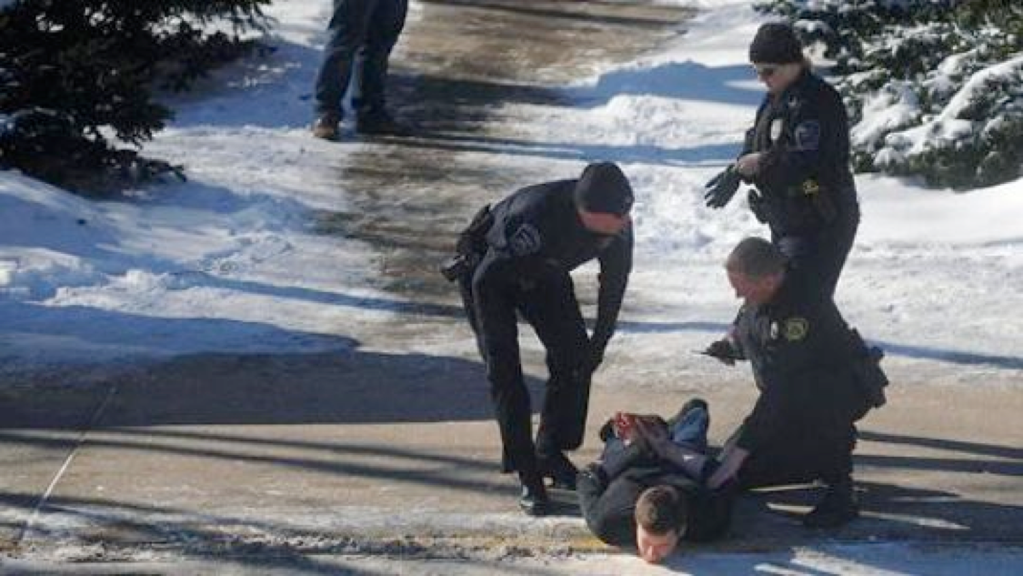
In January, 2014 there was a shooting at Purdue University, where one student entered a classroom and shot another student dead, then walked out and waited for police to arrest him.

At the time, it struck me that it was the third school shooting I had heard about in an approximately 10 day period.  Even for the United States, which has a serious problem with firearm violence compared to other first world countries, this seemed like an unusual number to have in such a short period of time.

It led me to wonder if perhaps contagion was playing a role in these dynamics.  Certainly, in the past it had been noted that suicide appears to be contagious, because (for example) in high schools where there is one suicide it is statistically more likely to see an ensuing cluster of suicides.  And the “copy cat” effect in mass killings has long been suspected.  I wondered if perhaps a mathematical model of contagion might be used to help quantify whether or not mass killings and school shootings are contagious.  So, I talked with some colleagues:

And, we decided to use a mathematical model known as a Hawke’s point process “self-excitation” model to simulate the potential dynamics of contagion in mass killings; the idea behind the model is quite simple… there is a baseline probability (which may or may not depend on time) of a mass killing to occur by mere random chance (the dotted line, below).  But, if a mass killing does occur, due to contagion it temporarily raises the probability that a similar event will occur in the near future.  That probability decays exponentially:

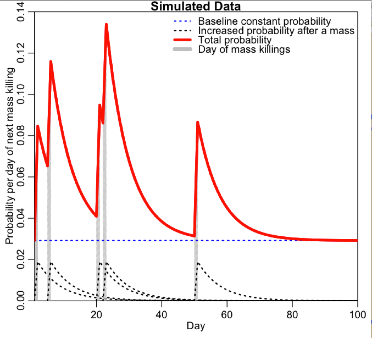
How contagion would manifest itself in data is thus as unusual “bunching together in time” of events compared to what you would expect from just the baseline probability.

Here’s our (blurry) model:

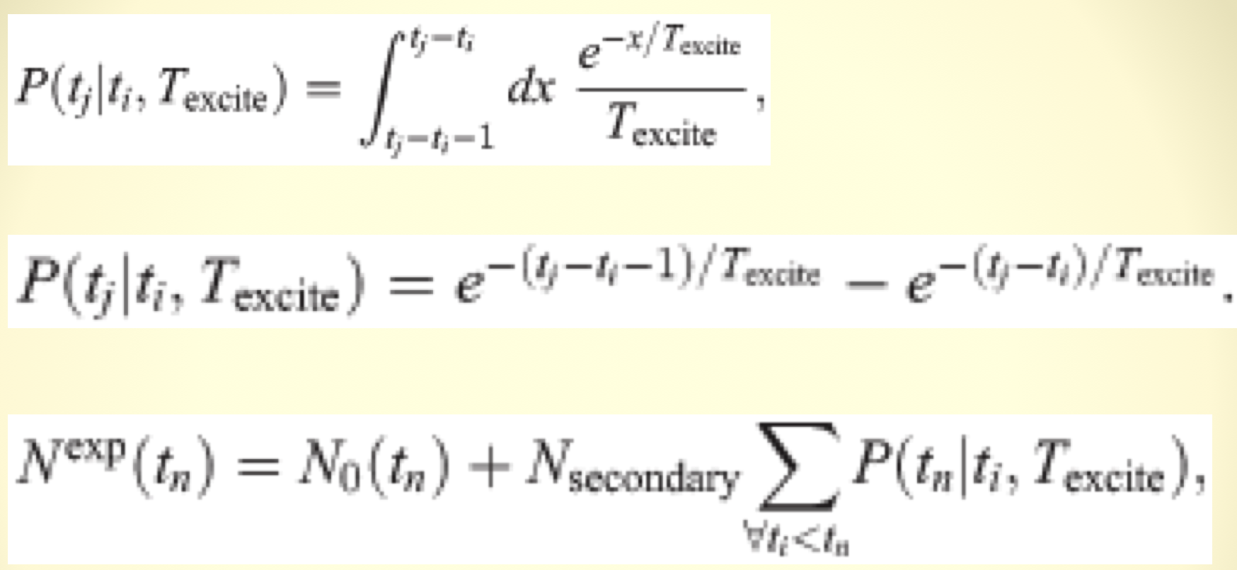
The parameters of the model were Texcite, the average length of the excitation period, and Nsecondary, the average number of new mass killings inspired by one mass killing.  N_0(t) was the baseline probability for mass killings to occur.  We used statistical modelling methods to estimate N_0(t).

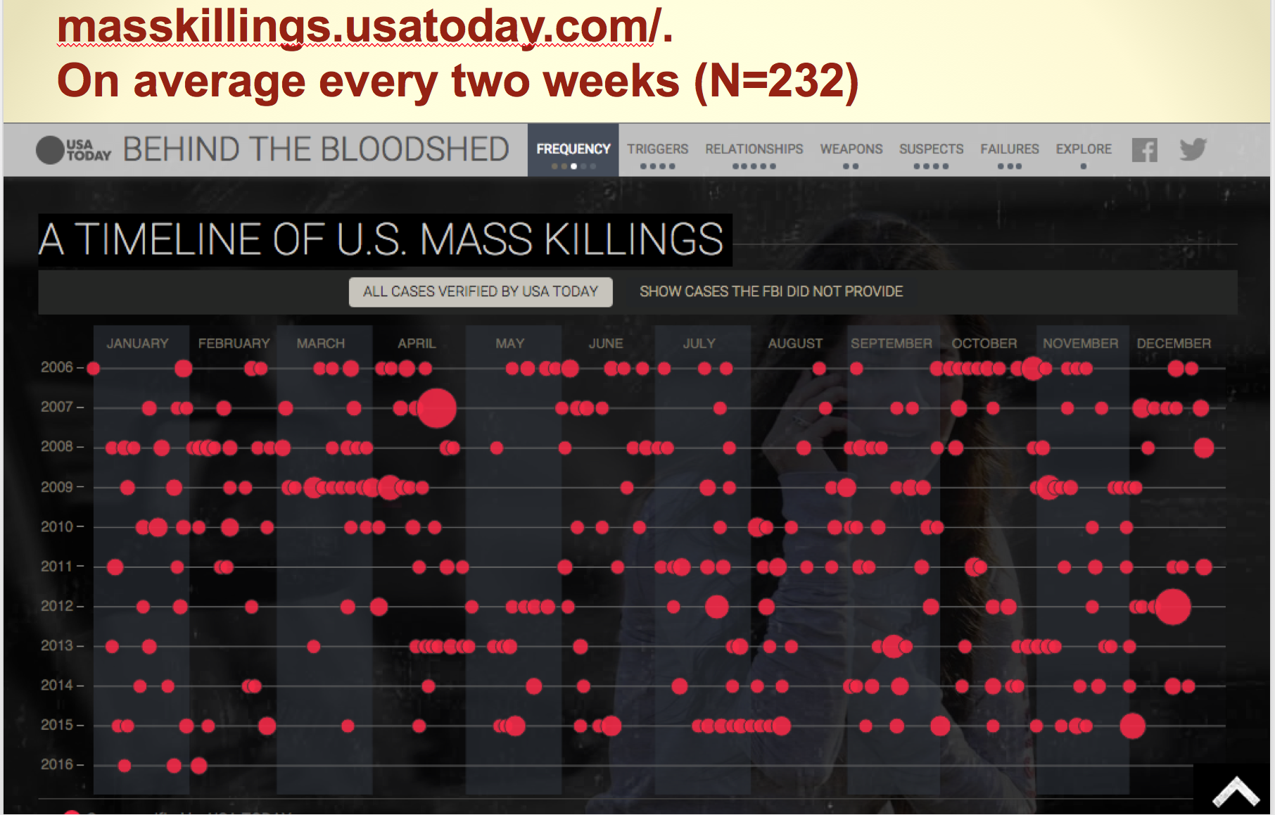
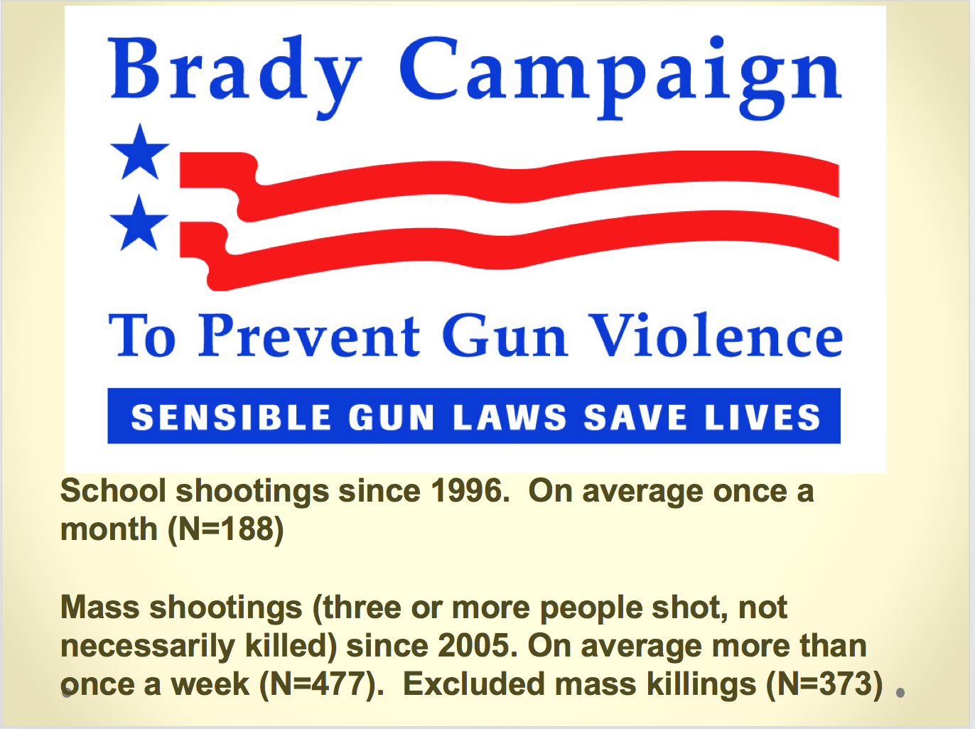
We needed data in order to fit the parameters of our model. From USA Today we obtained data on mass killings (four or more people killed), and from the Brady Campaign to Prevent Gun Violence, we obtained data on school shootings, and data on mass shootings (three or more people shot, not necessarily killed).  Mass shootings happen very frequently in the US!

We compared how well the Hawkes model fit the data compared to a model that didn’t include self-excitation.  If contagion is evident, the former will fit the data significantly better.

The fit results were:

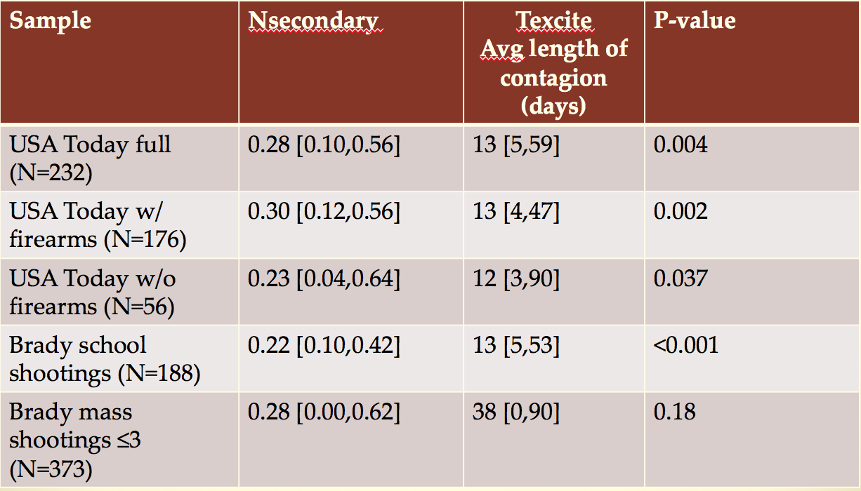
Both mass killings and school shootings appear to be significantly contagious!  And the length of the contagion period is on average around two weeks for both.

Mass shootings with more than three people shot, but less than four people killed were not contagious though.

Why?  Well, mass shootings with low death counts happen on average more than once a week in the US.  They happen so often, that they rarely make it past the local news.  In contrast, mass shootings with high death rates, and school shootings, usually get national and even international media attention.  It may likely be that widespread media attention is the vector for the contagion.

Again, this was an analysis that was made possible through the marriage of mathematical and statistical modelling methods.

Statistical and mathematical modelling skills on the job market

Quantitative and predictive analytics is a field that is growing very quickly.  Statistical methods and data mining (“big data”) play a large role in predictive analytics, but the power of mathematical models is more and more being recognized as having same advantages over statistical models alone because mathematical models do not simply assume an “X causes Y” relationship, but instead can describe the complex dynamics of interacting systems.  Having a tool box of skills that includes expertise in both mathematical and statistical modelling can lead to many interesting career opportunities, including consulting.