Archaeoastronomy: was the Merry Maidens site an astronomical observatory?

[This post is part of a series of posts on archaeoastronomy using open source software.  And, to ensure that readers are not kept in undue suspense as they read through the analysis below, the answer is: Yes, it does appear that the Merry Maidens site was used to observe the winter sun solstice, and also was apparently used as part of a larger ceremonial complex along with nearby neolithic sites as a lunar observatory]

Step 1: fit the lines between the stones

If I fit straight lines between the centers of all pairs of stones, even if I only take lines with angular uncertainty of less than 1/10th of a degree, we end up with a total of 167  site lines:

folly_b Continue reading

Archaeoastronomy: the folly of too many lines

[This post is part of a series of posts on archaeoastronomy using open source software]

In these modules, we’ve been considering the problem of archaeological sites that we posit may have been observatories of the rise/sets of celestial bodies. “Site lines” are lines drawn between salient features of a site that we posit might have been used to sight along to look at a particular point on the horizon.

Continue reading

Archaeoastronomy: where on the horizon do the stars, Sun, Moon rise and set? (Part II: correcting for the date the site was constructed)

[This post is part of a series of posts on archaeoastronomy using open source software]

In a previous post, we talked about the coordinate system of a person standing on earth observing a star (what the observer sees are the star altitude and azimuth), and how we can calculate the rise and set azimuths of stars/Sun/Moon at a given latitude if we know the equatorial declination coordinate of the star.  And we discussed that in the R file archeoastronomy_libs.R, there is a function called calculate_rise_set_azimuths() that will calculate the rise and set azimuths at a given latitude for a star with a given declination.

There are lots of places to look up catalogues of star declinations on the internet (for instance, here is one).  The SIMBAD astronomical database has a nice online query tool you can use to make your own custom list of stars. Continue reading

Archaeoastronomy: calculating the horizon profile using free online sources of digitized topographic data

[This post is part of a series of posts on archaeoastronomy using open source software]

In order to calculate where stars rise and set on the horizon at a particular location, we need to know what the horizon looks like at that place… are there mountains along the horizon?  If so, they can substantially change the rise or set azimuth of a star, compared to a flat horizon.

The website HeyWhatsThat allows you to enter the latitude and longitude and elevation of any location on earth, and get the horizon profile. Here is what the screen shot of the input page looks like:hey_whats_that_input

Continue reading

Archaeoastronomy: using R to fit straight lines between archaeological site datum points

[This post is part of a series of posts on archaeoastronomy using open source software]

After you have obtained a satellite image of an archaeological site, uploaded the image to the XFig graphical software package, and placed datum points on site features, you can get XFig to output the datum point coordinate information into a text file in Computer Graphics Metafile (CGM) format.

You can then use the free and open-source R statistical programming language to read in the CGM files and fit straight lines between the datum points. R is not only a programming language, but also has graphics and a very large suite of statistical tools. Connecting models to data is a process that requires statistical tools, and R provides those tools, plus a lot more.

Continue reading

Archaeoastronomy: using XFig to establish site datum points

[This post is part of a series of posts on archaeoastronomy using open source software]

Xfig is a free and open-source downloadable program for vector graphics widely used in physics.

In Xfig, I upload a satellite figure of an archaeological site, and then overlay circles over features in the site, trying to match as closely as possible their apparent diameter and position.

Continue reading

Archaeoastronomy: using Google Earth to obtain satellite imagery of archaeological sites

[This post is part of a series of posts on archaeoastronomy using open source software]

I use the free Google Earth software program to obtain satellite images of archaeological sites. If you download the Google Earth virtual globe program to your computer and start it up, in the search bar on the upper left hand side you can search for locations.

google_earth

Continue reading

Archaeoastronomy: a description of the UK Merry Maidens site

[This post is part of a series of posts on archaeoastronomy using open source software]

The Merry Maidens are a late neolithic ring of stones near St.Buryan in Cornwall in the UK, and is Cornwall Archaeological Unit site SW433245. The site consists of a circular ring of 19 upright stones, approximately 24 m in diameter, and is believed to be remarkably intact.  The stones are not large, with the largest being approximately 1.4m (just over 4 feet) tall. The site is believed to date from somewhere between 2500BC to 1500BC.

Here is a photo of the site (source www.ancient-wisdom.uk):


Continue reading

Archaeoastronomy: a short overview of my methodology using open source software

[This post is part of a series of posts on archaeoastronomy using open source software]

My work focusses on using Google Earth, a downloadable free virtual globe and geographic information program, to obtain satellite imagery of aerially-visible archaeological sites world wide that are suspected to have been used for astronomical observations, for instance stone circles and medicine wheels.  The uniqueness of my approach is that it does not require actually having to visit these sites in person to survey them. Continue reading

Some handy scripts and graphs for archaeoastronomy

If you are looking at an archaeological site that you believe was a comprehensive ancient sky observatory, it may be possible to date the site from its alignments to celestial phenomenon.  Note that you need a site with several likely sun/moon/star alignments to do this. On this page I provide some handy R and python scripts to calculate the rise/set azimuth (assuming a flat horizon) of the Sun, Moon, and stars for a given location at a given date.

Continue reading

Introduction to archaeoastronomy

Introduction

[This post is the first in a series on archaeoastronomy using open source software]

One of my academic hobbies is archaeoastronomy, which includes the study of how ancient peoples observed the sky.  As I will describe in a series of posts on this topic, I pursue my hobby with the use of free data and free software tools like Google Earth and the pyephem astronomical ephemeris calculation library, written in the Python programming language.

Continue reading

Research in archaeoastronomy using computational, mathematical, and statistical methods, with free and open source software

[On this page I document and describe some of my work in archaeoastronomy, using mathematical, computational, and statistical methods to rigorously assess the probability that an archaeological site was used as an astronomical observatory.  I will give, as an example, all the programming code and other files I used to analyze a stone circle in the UK known as the “Merry Maidens”.]


K-means clustering

Sometimes we may want to determine if there are apparent “clusters” in our data (perhaps temporal/geo-spatial clusters, for instance).  Clustering analyses form an important aspect of large scale data-mining.

K-means clustering partitions n observations into k clusters, in which all the points are assigned to the cluster with the nearest mean.

If you decide to cluster the data in to k clusters, essentially what the algorithm does is to minimize the within-cluster sum of squared distances of each point to the center of the cluster (does this sound familiar?  It is similar to Least Squares).

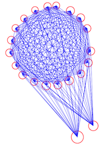
The algorithm starts by randomly picking k points to be the cluster centers.  Then each of the remaining points is assigned to the cluster nearest to it by Euclidian distance.  In the next step, the mean centroid of each of the clusters is calculated from the points assigned to the cluster.  Then the algorithm re-assigns all points to the their nearest cluster centroid.  Then the centroid of each cluster is updated with the new point assignments. And then the points are re-assigned to clusters.  And the cluster centroids re-calculated… and so on and so on until you reach a step where none of the points switch clusters. Visually, the algorithm looks like this:

How many clusters are in the data?

You likely want to explore how many distinct clusters appear to be in the data. To do this, you can examine how much of the variance in the data is described by our “model” (which in this case is the clustered data).  Just like for a linear least squares statistical model, we can thus calculate an adjusted R-squared from the total variance in the data and the sum of the within group variance.  There is also a way to calculate the AIC for a kmeans model.

To see how to implement kmeans clustering in R, examine the following code that generates simulated data in 3 clusters:

require("sfsmisc")
set.seed(375523)
n1 = 1000
x1 = rnorm(n1,100,5)
y1 = rnorm(n1,0,1)
n2 = 750
x2 = rnorm(n2,125,7)
y2 = rnorm(n2,4,0.5)
n3 = 1500
x3 = rnorm(n2,75,10)
y3 = rnorm(n2,-4,1)

x = c(x1,x2,x3)
y = c(y1,y2,y3)
true_clus = c(rep(1,n1),rep(2,n2),rep(3,n3))
pch_clus = c(rep(20,n1),rep(15,n2),rep(17,n3))
mydata = data.frame(x,y)
plot(x,y,col=true_clus,pch=pch_clus)

This produces the following plot:kmeans_1

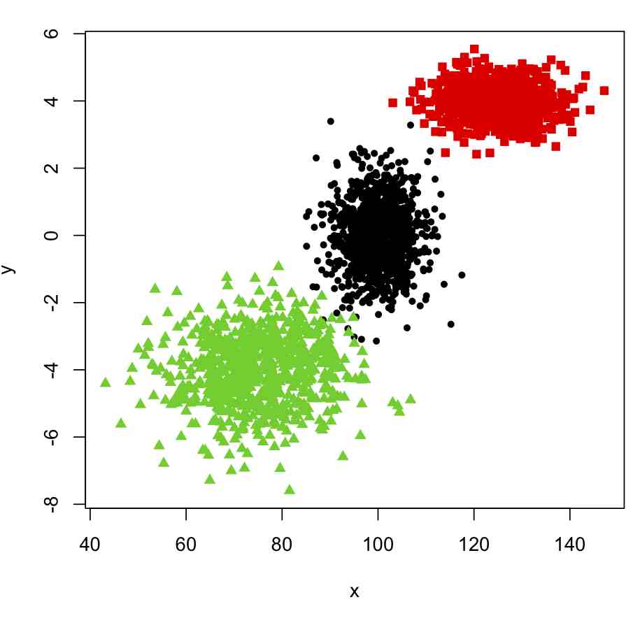
Now, to cluster these into nclus clusters, we can use the kmeans() function in R, like this

mydata_for_clustering=mydata
n = nrow(mydata_for_clustering)
nclus = 3
myclus = kmeans(mydata_for_clustering,centers=nclus)
print(names(myclus))

###################################################################
# plot the data, colored by the clusters
###################################################################
mult.fig(1,main="Simulated data with two clusters")
scol = rainbow(nclus,end=0.8) # select colors from the rainbow
plot(mydata$x,mydata$y,col=scol[myclus$cluster],pch=pch_clus)

Producing this plot:kmeans_2

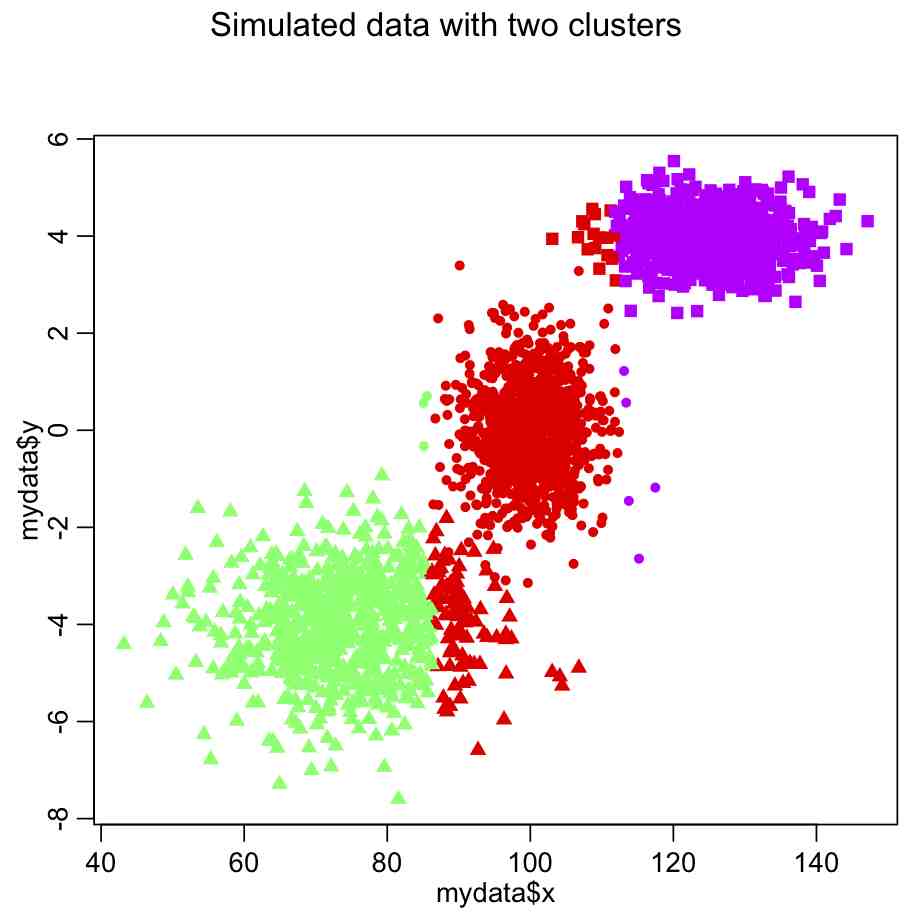
Do you see something wrong here?

The problem is that the x dimension has a much larger range than the y dimension, and so in the calculation of the Euclidean distance it carries far too much weight. The solution is to normalize the space such that all dimensions have the same dimensionality. Try this:

mydata_for_clustering=mydata
mydata_for_clustering$x = (x-mean(x))/sd(x)
mydata_for_clustering$y = (y-mean(y))/sd(y)
nclus = 3

myclus = kmeans(mydata_for_clustering,centers=nclus)
print(names(myclus))

###################################################################
# plot the data, colored by the clusters
###################################################################
mult.fig(1,main="Simulated data with two clusters")
scol = rainbow(nclus,end=0.8) # select colors from the rainbow
plot(mydata$x,mydata$y,col=scol[myclus$cluster],pch=pch_clus)

which yields the following:kmeans_3

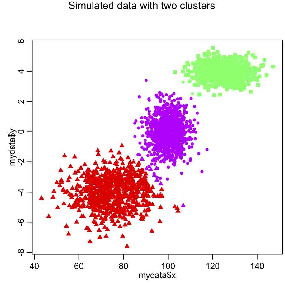
In most cases, however, the number of clusters won’t be so obvious.  In which case, we would need to use a figure of merit statistic like adjusted R^2 or (even better) AIC to determine which number of clusters appears to best describe the data.

To calculate the r-squared for a variety of cluster sizes, do this (after making sure your data are normalized!):

####################################################################
# the data frame mydata_for_clustering is ncol=2 dimensional
# and we wish to determine the minimum number of clusters that leads
# to a more-or-less minimum total within group sum of squares
####################################################################
kmax = 15 # the maximum number of clusters we will examine; you can change this
totwss = rep(0,kmax) # will be filled with total sum of within group sum squares
kmfit = list() # create and empty list
for (i in 1:kmax){
kclus = kmeans(mydata_for_clustering,centers=i,iter.max=20)
totwss[i] = kclus$tot.withinss
kmfit[[i]] = kclus
}

####################################################################
# calculate the adjusted R-squared
# and plot it
####################################################################
rsq = 1-(totwss*(n-1))/(totwss[1]*(n-seq(1,kmax)))

mult.fig(1,main="Simulated data with three clusters")
plot(seq(1,kmax),rsq,xlab="Number of clusters",ylab="Adjusted R-squared",pch=20,cex=2)

Producing the following plot:kmeans_4

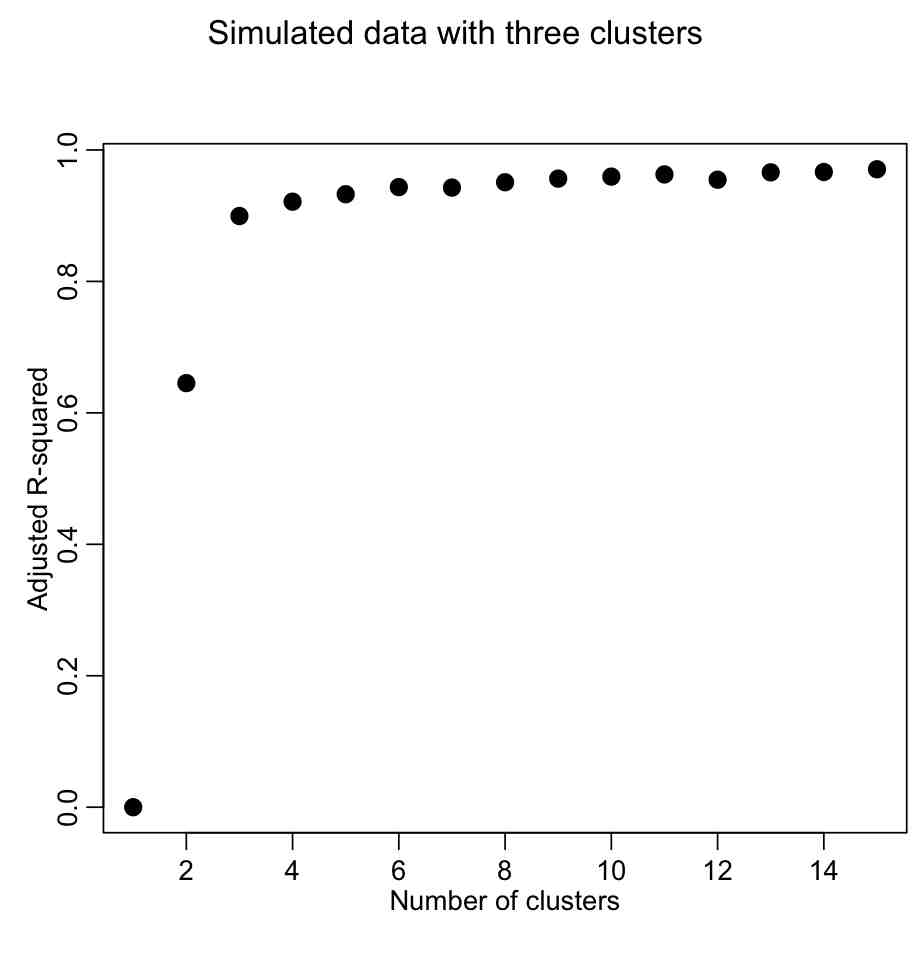
We want to describe as much of the R^2 with the fewest number of clusters.  The usual method is to look for the “elbow” in the plot, and that is traditionally done visually.  However, we could try to construct a figure-of-merit statistic that identifies the elbow.  In the AML610 course, the students and the professor developed a quantitative method to formulate a statistic to identify the elbow point.  We call this statistic the COMINGS-elbow statistic (after the first initials of the students who came up with the algorithm); the statistic looks for the (k,aic) point that has the closest euclidean distance to (1,min(aic)).  However, we noted that the performance of this statistic in identifying the elbow point was improved if we first normalized the k and aic vectors such that they lay between 0 to 1.  Thus, the elbow point is identified by the (k’,aic’) point that is closest to (0,0).

####################################################################
# try to locate the "elbow" point
####################################################################
vrsq = (rsq-min(rsq))/(max(rsq)-min(rsq))
k = seq(1,length(vrsq))
vk = (k - min(k))/(max(k)-min(k))
dsq = (vk)^2 + (vrsq-1)^2

cat("The apparent number of clusters is: ",nclus,"\n")
points(nclus,rsq[nclus],col=2,pch=20,cex=2)

This figure-of-merit for elbow location doesn’t seem to work optimally. Can we think of a better one?

The AIC can be calculated with the following function:

kmeansAIC = function(fit){

m = ncol(fit$centers)
n = length(fit$cluster)
k = nrow(fit$centers)
D = fit$tot.withinss
return(D + 2*m*k)
}

aic=sapply(kmfit,kmeansAIC)
mult.fig(1,main="Simulated data with two clusters")
plot(seq(1,kmax),aic,xlab="Number of clusters",ylab="AIC",pch=20,cex=2)

Again, we are looking for the elbow point in the plot.

####################################################################
# look for the elbow point 
####################################################################
v = -diff(aic)
nv = length(v)
fom = v[1:(nv-1)]/v[2:nv]
nclus = which.max(fom)+1
cat("The apparent number of clusters is: ",nclus,"\n")
points(nclus,aic[nclus],col=2,pch=20,cex=2)

This yields:kmeans_5

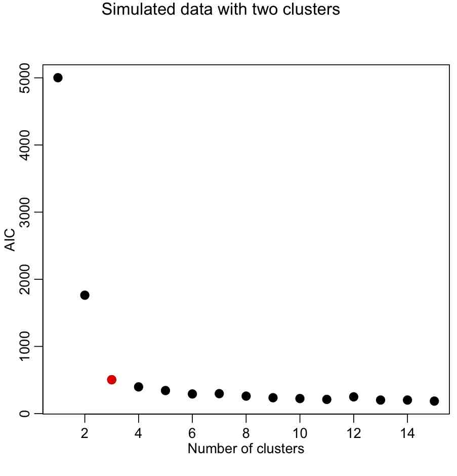
With the AIC, our elbow locator FoM seems to work better (in this case, anyway).

In the file kmeans_example.R, I show the location of terrorist attacks in Afghanistan between 2009 to 2011 from the Global Terrorism Database.   The data are in afghanistan_terror_attacks_2009_to_2011.txt

One sided vs two-sided tests

In this course so far we have covered the Z-test, the Student’s-t test and the chi-square test for testing the null hypothesis “is quantity A consistent with quantity B”.

The Z and students-t statistics are examples of two-tailed statistics, because two directions are considered “extreme”; the far low end and the far high end.  If your Z statistic is very low or very high, you would conclude that you should reject the null hypothesis that A is consistent with B:

File:P-value Graph.png

So far in this course, I’ve told you that if the p-value of the Z or students-t statistic returned by the pnorm() or pt() functions in R is less than 0.05, or greater than 0.95 (ie; p<0.05 or (1-p)<0.05), you probably should reject the null hypothesis that A is consistent with B.  Some people use a more stringent test, where they reject the null if p<0.025 or (1-p)<0.025.  The value on the RHS that is used as the cut-off value for p is known as the “critical value”, and is often denoted as alpha.


Using the chi-squared statistic to test if two Normally distributed variables A and B are statistically consistent with being equal to each other with a critical value of p<alpha* is exactly equivalent to using the two-sample Z test for the equivalence of A and B, with a critical value p<alpha/2 (or (1-p)<alpha/2)**.

* recall that if you use the pchisq() function in R, then the p-value of the test statistic is p=1-pchisq()

** recall that if you use the pnorm() function in R, then if pnorm()<0.5, the p-value of the test statistic is p=pnorm().  If pnorm>0.5 then the p-value of the test statistic is p=1-pnorm().

If you use this more

mple of a one-tailed


test because only one end is considered as “extreme”